Density estimation with kernels

PDFs and parametric vs. non-parametric approaches

When analyzing a set of data, it may be useful to determine the underlying probabalistic process (assuming one exists) that generated said data. That is, assume for a data set $x_i\in \mathbf{x},i=1,\dots ,n$, with $\mathbf{x}$ realizations of a random variable $X$, the probability data falls within an interval $[a,b]$ is given by

$$P(a<x<b)={\int }_b^{a}f(x)dx$$

The function $f(x)$ is known as the Probablity Density Function (PDF). Obtaining an appropriate estimate for $f(x)$ on a data set will in turn be an estimate of the data-generating process behind said data. For example, the below plot is the PDF of the standard normal distribution.

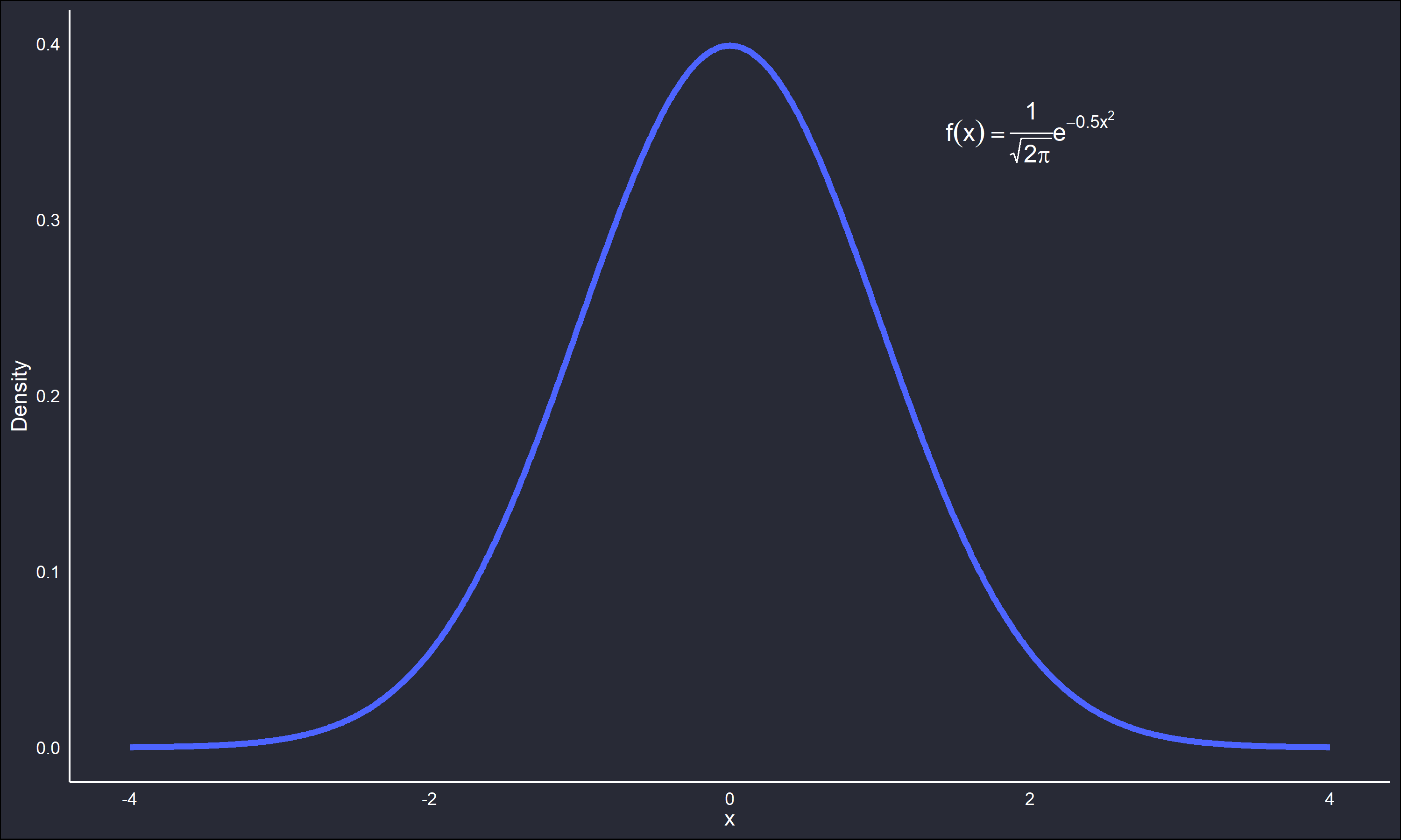
The scale parameter (variance) is 1 and the location parameter (mean) is 0. A set of data theorized to come from this distribution would have the majority of values about 0, and few outliers beyond the upper and lower tails.

How to obtain an estimate $\hat{f}(x)$ for $f(x)$? A common approach is to study the data and assume a parametric distribution , then estimate parameters for said distribution from the data. However, it may be undesirable to make a parametric assumption over the data for some research domain reason. Lacking a specific external reason to not make a distributional assumption, it may still be desirable as a matter of principle to not make a potentially restrictive assumption. Methods that relax or eliminate distributional assumptions fall under a statistical sub-topic known as non-parametric statistics. A well studied approach to estimating $\hat{f}$ with non-parametric methods is Kernel Density Estimation (KDE).

The kernel approach

To better contextualize KDE, consider the histogram. A histogram is a tried and true method of data visualization, however it also can be thought of as a crude approximation of a PDF. Below is a histogram for 10,000 datapoints sampled from the previously mentioned normal distribution, with a bin width of 0.5 units.

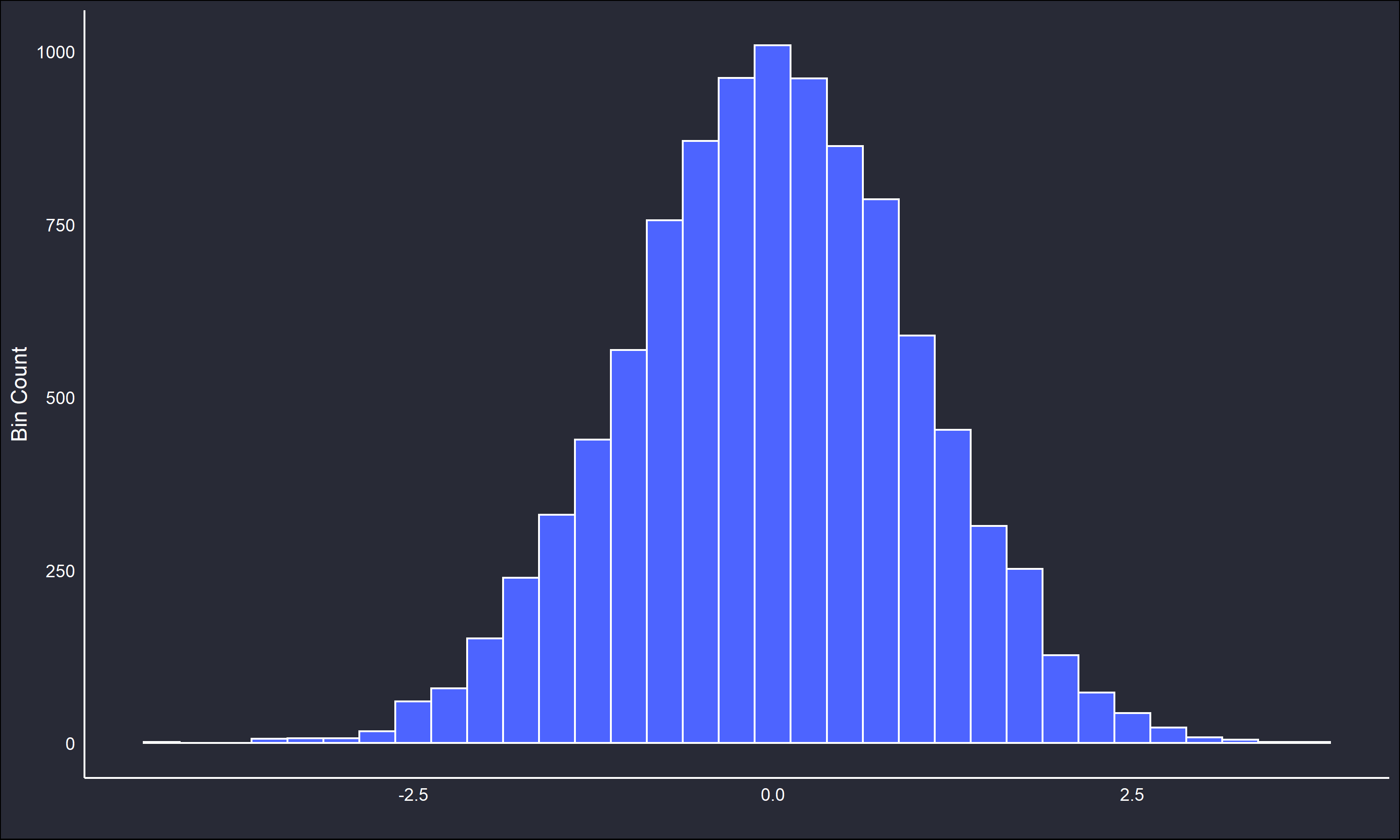
Note how the unimodality and symmetry from the standard normal PDF is reflected in the histogram. The histogram is an excellent tool for exploratory analysis, however it is not without shortcomings. Changing the bin width or origin may greatly affect the interpretation of the histogram. Further, the histogram as an estimate of a PDF is not mathematically suitable. The bin counts may be transformed into density estimates, however the underlying function has none of the properties of a PDF, for example differentiability and integration to unity. This can be problematic depending on the reasons for estimating $\hat{f}$

The KDE approach differs from the histogram to address these concerns. Instead of representing density by the proportion of data occupying a discrete set of bins of fixed width, an individual function is affixed to every data point. The individual curves are then summed together into a single smooth estimate of $\hat{f}$. Formally,

$$\hat{f}(x)=\frac{1}{nw}\sum _i^{n}K(\frac{x-x_i}{w})$$

where $K$ is a function typically chosen to be a unimodal symmetric PDF itself, $n$ is the sample size of the data, $w$ is a smoothing parameter somewhat analogous to the bin width of a histogram, and $x_i$ are the considered data points. A simple example with only 5 data points is used to illustrate KDE, actual density estimation on samples of such low size is innapropriate.

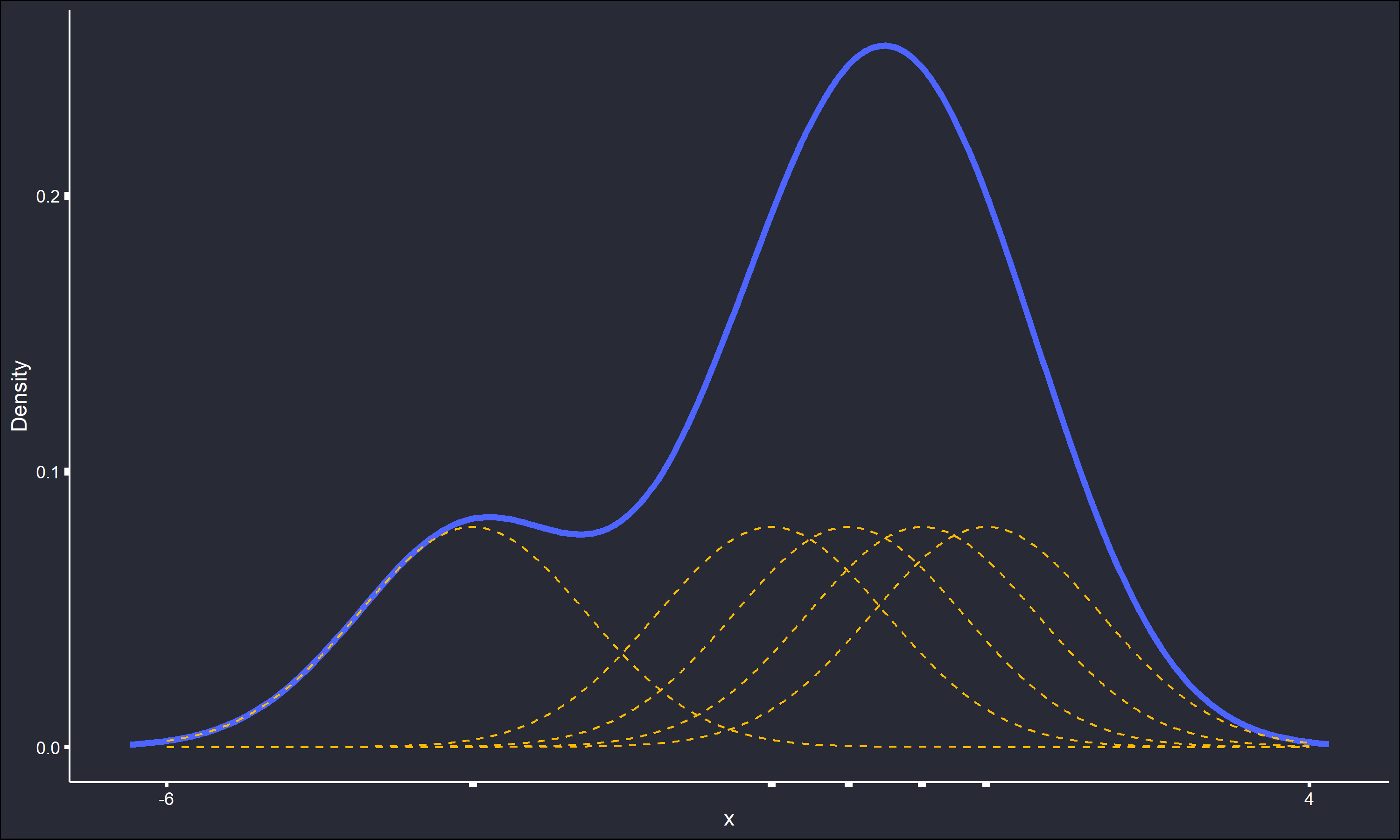
The $K$’s are normal PDFs and the smoothing parameter $w$ is set to 1. It is easy to see how the dashed indivdual kernels sum into the overall density estimate. The same process is repeated, except with $w=5$.

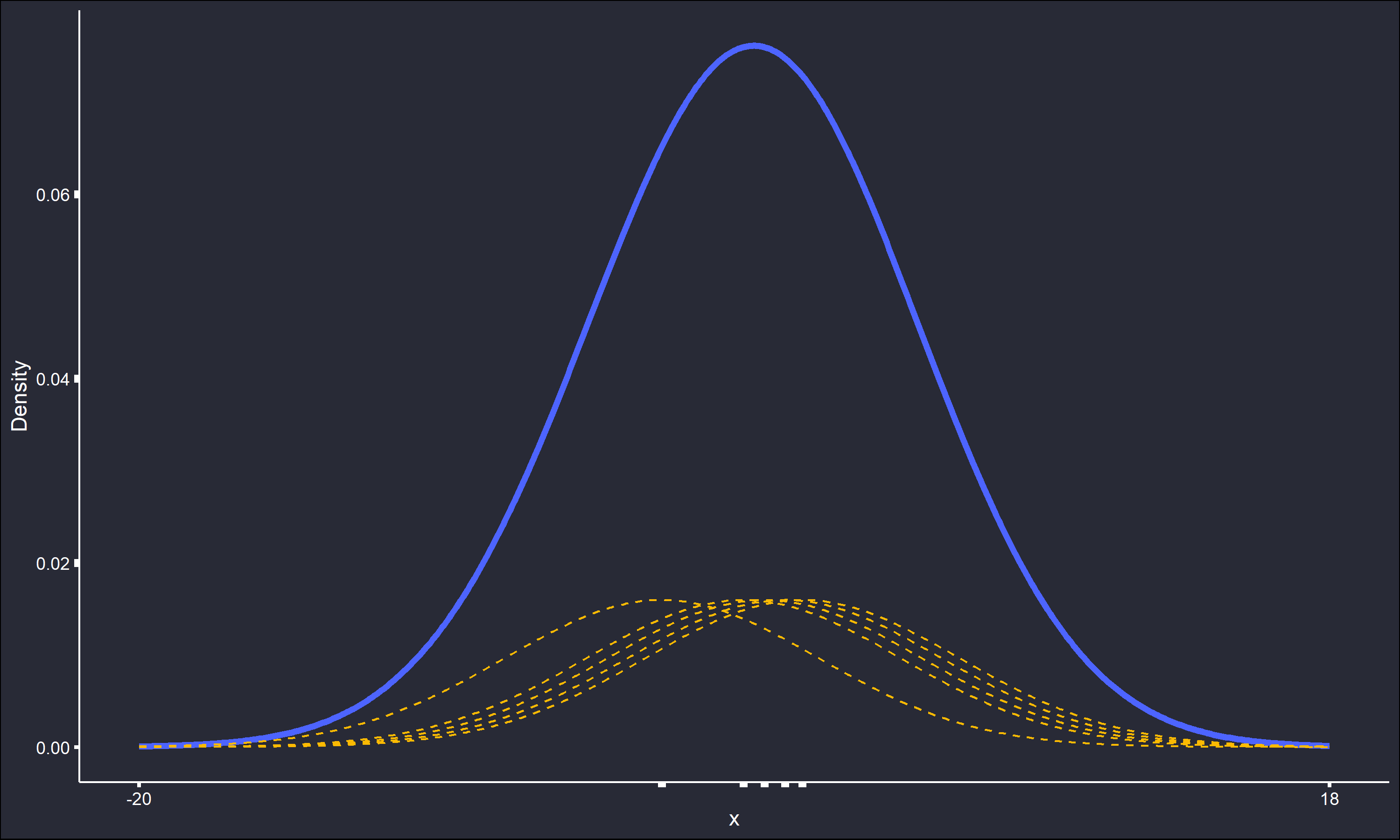
All the detail in the estimate has been smoothed out, and the absolute range of the estimate has also increased over 300%. Cleary the value of $w$ can be extremely important in determining the shape of the density estimate. In contrast, the selection of $K$ is well known in the literature to be far less relevant to the final estimate within the KDE process. Unless there is a good domain-specific reason for another selection, sticking to a choice of $K$ that is symmetric, unimodal, and has any desired properties of a PDF, is acceptable.

There exist iterative methods for the “optimal” selection of $w$, as well as some accepted rule of thumbs. A thorough discussion on the selection of $w$ is beyond the scope of this post, but a good starting point for the interested reader would be the paper Density Estimation (Sheather, 2004).

Note that straightforward KDE is not without it’s shortcomings. In particular, every data point is affixed with a kernel weighted and shaped the same regardless of the relative “closeness” of the data. That is, outliers or other information in the tails may be given too much importance in the final estimate. There do exist adaptive methods to address this issue that essentially let $w$ become some function of the “closeness” of each data point to others. An excellent (but somewhat old) overview of density estimation with kernels is the monograph Density Estimation for Statistics and Data Analysis (Silverman, 1986), which does a good job of introducing and expanding upon these ideas.

KDE as explained here is a relatively simple process, but matters can become more complex. Either of the two sources I reccomended above would be a good way to become more aquainted with these details. I hope this post serves as a good starting point to this useful topic.