Using permutation tests with a simple dataset
Permutation tests (aka randomization tests) are a non-parametric way to conduct a statistical test. Parametric tests will require assumptions to be made about the data being analyzed that may be difficult to justify. Strict assumptions may be relaxed by appealing to asymptotic results, but this will not always be possible or desirable.
Many well-known statistical tests of comparison will assume the data are independent draws from a known probability distribution. This assumption may be difficult to approximate in real life situations, much less guarantee. For the experimenter, it is typically much easier to have a non-random sample of data, but assign treatments and/or controls randomly. Permutation tests are especially useful in this arena.
Hypothesis tests and exactness
Under the widely used Neyman-Pearson paradigm of statistical hypothesis testing, there is a null hypothesis and an alternative hypothesis. There are other paradigms, but for simplicity we are focusing on this one. Inherent to every test is the possibility of error. The probability of rejecting a true null is known as Type I error, the probability of failing to reject a false null is known as Type II error. Of course it would be best to minimize both Type I and Type II error, however this is not feasible as the errors have a complementary role (consult any textbook/resource on introductory statistical inference to see why). That is \(P(\mathrm{Type \ I})\) increases as \(P(\mathrm{Type \ II})\) decreases. Most researchers and experimenters design their methods such that they seek to reject a null in favour of an alternative, but this leads to Type I error being the more concerning of the two since it can undermine the entirety of the research objectives. In order to address the problem of the symmetric relationship between Type I and II error, asymmetry will be deliberately introduced in the form of a pre-determined significance level \(\alpha\), representing \(P(\mathrm{Type \ I})\). This probability will be set low (relative to the research domain), and then a test will be constructed/chosen such that \(P(\mathrm{Type \ II})\) is minimized.
I’ll skip over the mathematical details as there are many resources easily available covering that in varying depth. However the following diagram illustrates the ideas nicely.
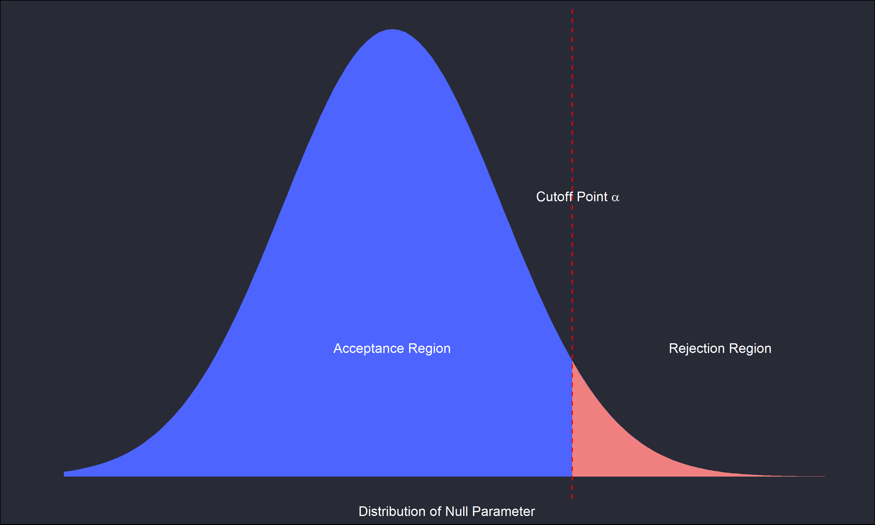
This is a one-sided test, where any values of the parameter of interest left of \(\alpha\) means we fail to reject the null hypothesis, and any value to the right of \(\alpha\) means a rejection of the null. It is important to re-emphasize the selection of \(\alpha\) is subjective and possibly specific to the research domain. For example, in testing materials used to build an airplane \(\alpha\) may need to be extremely low relative to some variable in an observational study.
An exact test will guarantee control over testing error. That is, an error level \(\alpha\) determined ahead of time is guaranteed to be equivalent to \(P(\mathrm{Type \ I})\). Straightforward parametric tests may only offer exactness under restrictive assumptions. The potential for the actual error to exceed the prescribed error level may be problematic. In contrast, permutation tests offer control of error with (relatively) easy restrictions for the researcher, randomizing treatments and controls over subjects.
Permutation test under a randomization model
A permutation test will differ from a parametric test through the frequency distribution underlying the null hypothesis. In a typical parametric test a distribution is assumed across the test parameter from domain knowledge or the data itself. In contrast, the permutation method will generate a discrete empirical distribution for the test statistic from the data. There are two broad models under which to consider a permutation test: a population model and a randomization model. Permutation tests under a population model (assuming the data are random samples) have natural competition from more well known parametric alternatives. Under the randomization model the only assumption needed is that treatments and/or controls were applied randomly to subjects in an experiment (obviously the data being from an experimental design is itself a requirement!). In many experiments it is far easier to guarantee random assignment of treatments and/or controls than a true random sample of the data from a population. Hence the randomization model is (to me) a more compelling application of permutation tests, since the more well-known parametric tests may be undesirable (theoretically, if not practically) in light of difficulties to obtain an actually random sample.
Moving forward with the randomization model, I will use the chickwts dataset from R. In this dataset, a very simple experiment was conducted such that 72 newborn chicks were randomly assigned a variety of different feed supplements, and their weights in grams were measured six weeks later.
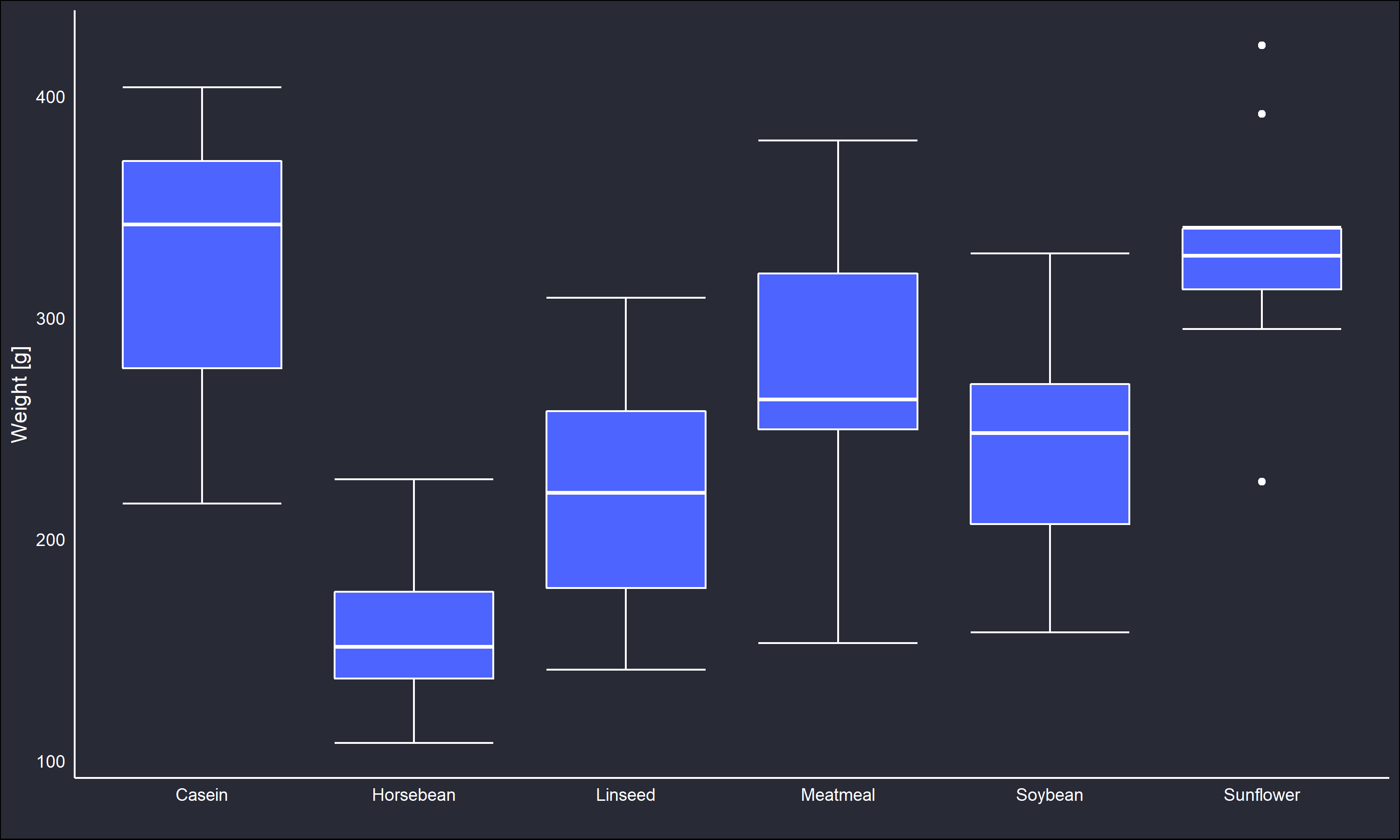
The boxplot indicates the feedtypes resulted in fairly different distributions of weights for the chicks. However, soybean and linseed seem to be the closest. Suppose we are interested in evaluating whether the difference between soybean and linseed can be attributed to random variation or not. Then,
\[\begin{aligned} H_0: \bar{X}_{\mathrm{soy}} &= \bar{X}_{\mathrm{lin}} \\ H_A: \bar{X}_{\mathrm{soy}} &\neq \bar{X}_{\mathrm{lin}} \end{aligned}\]There are of course statistics other than the mean that can be used to evaluate a difference between groups.
How to develop a reference distribution for \(H_0\) with non-parametric methods? Note that our null assumption is that soybean and linseed have the same effect on a chicks weight after 6 weeks. Logically it makes sense that under this assumption, any given assignment of soybean or linseed feed to those chicks would result in the same test statistic. Hence a null distribution may be obtained through calculating all possible ways to assign the soybean and linseed to the chicks.
In this data there are 12 chicks with linseed feed, and 14 with soybean feed. The total number of ways the feeds could have been assigned is then \({26 \choose 12} \approx 9.7\times10^6\). This number is large, but not impractical to work with given modern computational power. However, it is obvious for larger experiments exactly calculating all the permutations of the test statistic is impractical. In situations with larger samples the reference distribution can be generated through Monte Carlo sampling.
Another way to reduce computational resources is a transformation of the test statistic. In this example, calculating both \(\bar{X}_{\mathrm{soy}}\) and \(\bar{X}_{\mathrm{lin}}\) may be tedious (both to execute and code). However \(\bar{X}_{\mathrm{soy}} - \bar{X}_{\mathrm{lin}}\) can be represented as a function of \(\sum_i^n X_{i,\mathrm{lin}}\). To see this,
\[\begin{aligned} \bar{X}_{\mathrm{soy}} - \bar{X}_{\mathrm{lin}} &= \bar{X}_{\mathrm{soy}} - \bar{X}_{\mathrm{lin}} + \frac{\sum_i^n X_{i,\mathrm{lin}}}{m} - \frac{\sum_i^n X_{i,\mathrm{lin}}}{m}\\ &= (\bar{X}_{\mathrm{lin}} + \frac{\sum_i^n X_{i,\mathrm{lin}}}{m}) - (\bar{X}_{\mathrm{soy}} + \frac{\sum_i^n X_{i,\mathrm{lin}}}{m})\\ &= \frac{m+n}{mn}(\sum_i^nX_{i,\mathrm{lin}}) - \frac{1}{m}(\sum_j^mX_{j,\mathrm{soy}} + \sum_i^n X_{i,\mathrm{lin}}) \end{aligned}\]where \(m=14\) and \(n=12\). Note \(\sum_j^mX_{j,\mathrm{soy}} + \sum_i^n X_{i,\mathrm{lin}}\) does not change regardless of the random assignment. It is clear from some more straightforward algebra that \(\sum_i^nX_{i,\mathrm{lin}}\) is a function of \(\bar{X}_{\mathrm{soy}} - \bar{X}_{\mathrm{lin}}\), and is independent of any random assignment. Hence \(\sum_i^nX_{i,\mathrm{lin}}\) will be a test statistic that preserves the ordering of \(\bar{X}_{\mathrm{soy}} - \bar{X}_{\mathrm{lin}}\), and thus can be used to generate equivalent statistical conclusions.
The next step is to generate the reference distribution of the statistic.
#Get data
require(datasets)
dat1 = chickwts

#subset data to get variables we want
redDF = rbind(subset(dat1, feed=='soybean',select = c('weight','feed')),
              subset(dat1, feed=='linseed',select = c('weight','feed')))

#Exhaustive generation of reference distribution
combsSum = (combn(redDF$weight, 12, FUN = sum)) #apply sum over all ways to assign 12 from 26

#Monte-Carlo sampling to generate reference distribution. Use 10000 samples
MCsamp <- replicate(10000, {
  ss = sample(redDF$weight, size = 12 ,replace = F)
  sum(ss)
})
The below figures compare the two reference distributions.
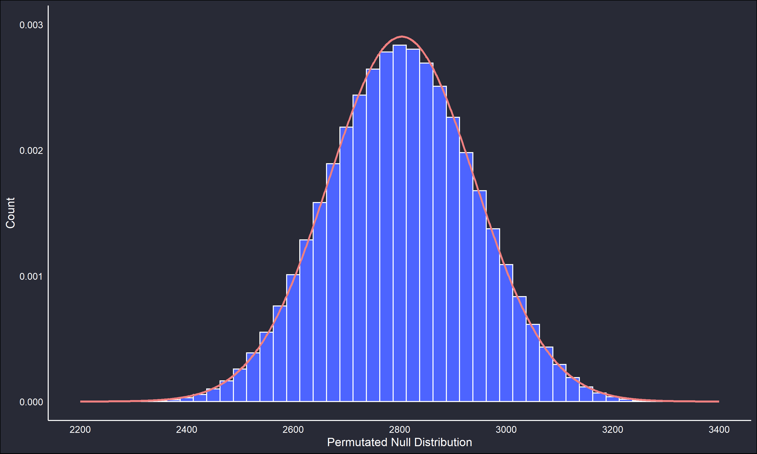
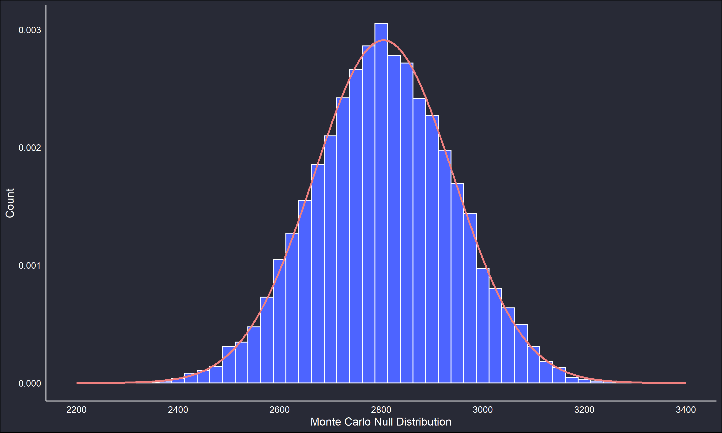
The permutated null distribution is very unimodal and symmetric. However, the Monte Carlo null distribution retains enough of the main features of the permutated null to be useful. The fitted lines on the null distributions are a normal distribution parametrized by the maximum likelihood estimates (sample mean and variance) of the generated data. The fitted parametric distribution is a very close fit to the non-parametric reference distribution in both cases, but we’ll continue working with the non-parametric distribution.
The test statistic \(\sum_i^nX_{i,\mathrm{lin}}\) for the observed data is \(2625\). Under the null hypothesis, this value is just one permutation of many, equally possible assignments. Hence a one-sided p-value can be calculated as the number of permutated test statistics less than or equal to the observed test statistic, scaled by the total number of possible permutations. For the Monte Carlo sample this is amended simply by scaling by the number of re-samples instead.
\[\begin{aligned} p_{\mathrm{Monte \ Carlo}} &= P(\sum_i^{10000} X_{i,\mathrm{lin}} \leq 2625 | H_0) = \frac{\sum_i^{10000}I(X_{i,\mathrm{lin}} \leq 2625)}{10000} = 0.0984\\ p_{\mathrm{Permutated}} &= P(\sum_i^{26\choose12} X_{i,\mathrm{lin}} \leq 2625 | H_0) = \frac{\sum_i^{26\choose12}I(X_{i,\mathrm{lin}} \leq 2625)}{26\choose12} = 0.0994\\ \end{aligned}\]Both p-values show moderate evidence to reject the null hypothesis, and both p-values are very close to each other, further illustrating the usefulness of the Monte Carlo process. There is a roughly 10% chance the observed difference in chick weights from linseed and soybean supplements is due to randomness in the assignment of the feed supplements, and not because of a difference between the feed types ability to affect growth.
Depending on the research context that may be sufficient to argue for the soybean supplement growing heavier chicks, or it may not. If \(\alpha\) is chosen such that it is a multiple of \({26\choose12}^{-1}\) then the test is exact due to the discreteness of the non-parametric reference distribution. If \(\alpha\) is not a multiple of \({26\choose12}^{-1}\), then the closest value of \({26\choose12}^{-1}\) less than \(\alpha\) will be a conservative estimate of \(P(\mathrm{Type \ I})\). Regardless the permutation test offers guarantees of the control over error that may be harder to achieve in parametric alternatives. The generalizability of this framework and notation should be clear.
I will leave it there for now, but there is much more than can be said about permutation tests and the ways to apply them. A couple good references I saw recommended on the Cross Validated stack exchange were Permutation Methods: A Basis for Exact Inference (Ernst 2004) and Why Permutation Tests are Superior to t and F tests in Biomedical Research (Ludbrook & Dudley 1998), and I can confirm they are both readable and interesting explanations of the topic.