Chess checkmates - A simple neural network

Introduction

Chess is an ancient and complex game, humans have been playing chess and chess variants for thousands of years. I began playing chess somewhat seriously around 2015, and it has quickly become one of my favourite games. You can find a good primer for learning the rules of chess here.

Hobbyists, scientists, and professionals have sought to look deeper into the nature of chess and explore it’s complexities for many years. A natural course of study was to program computers to be able to play chess against humans and, eventually, beat them. This work reached a seminal moment in 1997 when IBMs Deep Blue supercomputer defeated the world champion of chess Garry Kasparov in a series of 6 games. From then on chess engines only became stronger. Nowadays all top chess engines could easily defeat any human.

However, how typical chess engines play chess is very unlike how humans play. A chess engine such as Stockfish or Komodo will play chess through sheer calculation. That is, chess engines will utilize a computers ability to perform many ordered tasks quickly and efficiently to calculate the strength of thousands of series of moves in any given position, and then choose the best option. Such a strategy is far beyond any humans ability. Strong human chess players will choose their moves through a combination of experience, intuition, and manual calculation.

In the past several years chess engines have been developed that do not rely purely on brute force calculation. The DeepMind company developed a program called AlphaZero that has mastered chess (along with go and shogi) through neural networks (NNs). A similar neural net based program, Leela Chess Zero, is open source and is an ongoing project.

All of this recent work involving neural net based chess engines, as well as the (relatively) recent explosion of interest in artificial intelligence (AI) and deep learning, piqued my interest in further applications of AI in chess.

A particularly popular application of NNs is image classification, that is training a model to accurately predict a label across a given set of images. I have experience working with large sets of images for statistical applications before, and thought it would be fun to investigate a NN applied to large sets of chess images. I figured checkmates would be promising as a starting point. In chess, checkmate is the win condition of the game. It is achieved when a player’s king is attacked by an opposing piece, and every accessible adjoining square the king may move to is also attacked by an opposing piece.

The black king is attacked by the white queen, and his escape route via f7 is controlled by the white pawn on e6

I decided upon investigating checkmates because of their inherent simplicity. Any given chess position is either checkmate or not checkmate. This is a binary outcome, and binary classification is a well studied application of NN modelling. My background is in math and statistics, but I have no formal training in AI and machine learning and have devoted little independent study to the field, so starting simple seems like a good idea.

Part One - Data sourcing and cleaning

After deciding what I wanted to investigate, I needed to figure out a way to obtain the necessary data. My initial idea was to just surf the internet for random repositories of checkmate positions in FEN files, which could then be used to generate images. However I quickly discovered two problems.

1. It is somewhat difficult to find repositories of FEN files that are of an actual checkmate.
2. After locating a repository there were far too few actual positions! Image classification needs many many images for training and subsequent validation.

My next idea was to obtain a large dataset of chess games, identify which games ended in a checkmate position, and extract those positions to generate images. Enter lichess. Lichess is a completely free and open source chess website, and I highly recommend it if you are interested in playing online chess. Lichess conveniently archives every single game played on their site by month, with games as far back as 2013. To reduce computing time, I chose the month with fewest games, January 2013, during which a mere 121,332 games were played.

An aside, to give you an idea of how popular lichess has become over the years I scraped the number of standard (non-variant) games played per month.

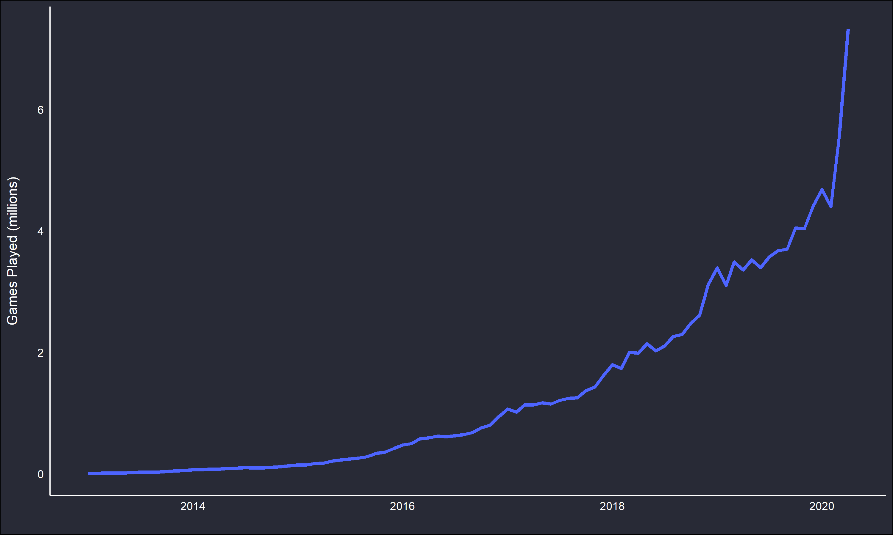
The huge spike at the end is due to the ongoing covid-19 global pandemic.

Moving on, the games are bundled into a single .bz2 file, and are all in PGN format. After I downloaded the January 2013 file I needed a way to parse through the games and extract desired features. I decided to use the python library python-chess as it was recommended on the lichess game archive.

I don’t have a ton of experience working with python, so I am sure my approach is by no means the best or most efficient.

#load library
import chess.pgn 

#store downloaded pgn file
pgn = open("lichess_db_standard_rated_2013-01.pgn", encoding="utf-8-sig")

We can look at all the categories in a game from the pgn file.

chess.pgn.read_headers(pgn)

## Headers(Event='Rated Classical game', Site='https://lichess.org/j1dkb5dw', White='BFG9k', Black='mamalak', Result='1-0', BlackElo='1403', BlackRatingDiff='-8', ECO='C00', Opening='French Defense: Normal Variation', Termination='Normal', TimeControl='600+8', UTCDate='2012.12.31', UTCTime='23:01:03', WhiteElo='1639', WhiteRatingDiff='+5')

The goal is to extract positions with checkmate on the board. Lichess tags games that end in resignation or checkmate as “Normal” termination in pgn files. The initial parse will identify the locations of all these games across the main .pgn file.

#Create empty array to store games that ended in checkmate
checkmate_games = []

#1st parsing: get game locations that end normally
while True:
    offset = pgn.tell() #stores current file position
    headers = chess.pgn.read_headers(pgn) #stores current header
    
    if headers is None: #if no value go to next file location
        break
    if "Normal" in headers.get("Termination"):
        checkmate_games.append(offset)

Now that we have the file locations of games that ended normally, we need to store the actual games.

#2nd parsing: get games that ended normally
checkmate_games2 = []

for i in checkmate_games:
    pgn.seek(i)
    checkmate_games2.append(chess.pgn.read_game(pgn))

Now that we have stored all the actual games that ended normally, we need to find the subset of games that ended in checkmate.

#3rd parsing: get games that end in checkmate
checkmate_games3 = []

for i in range(len(checkmate_games2)):
    if(checkmate_games2[i].end().board().is_checkmate()):
        checkmate_games3.append(checkmate_games2[i])
        
len(checkmate_games3)

34474

Out of the initial 121,332 games in the file only 34,474 ended in checkmate.

The NN that will be trained still needs inputs, the next step is to get the checkmate positions in all 34,474 games and store these positions as images. Fortunately the python-chess library has a module that suits our needs, and will create an svg image of a specified chess position.

#Write an svg image of every checkmate position to disk
for i in range(len(checkmate_games3)):
    outfilename = '%smate.svg' % (str(i)) #create unique file name, e.g. 0mate.svg, 1mate.svg, ...
    outputFile = open(outfilename, mode = "w")
    outputFile.write(chess.svg.board(board = checkmate_games3[i].end().board(), coordinates=False))
    outputFile.close()

The .end() method will grab the position at the end of a game, .board() will generate a board representation for chess.svg.board() to render.

Now all the checkmate positions are saved as images as desired. However in order to train the NN, we will need more than just checkmate positions. To get chess positions that are not checkmate positions I looped through the stored games that ended normally, and extracted a random position from the game (that wasn’t checkmate), then saved that position again as a svg file.

import random as ran

for j in range(1,73552):

    board1 = checkmate_games2[j].board() #store jth game as a board
    moves = []
    
    
    for move in checkmate_games2[j].mainline_moves(): #append move list
        moves.append(move)
    
    if(len(moves) - 2 <= 1): #filter games that end after 2 moves or less
        continue
    
    r1 = ran.randint(1,len(moves)-2) #random total number of moves that won't result in checkmate.
    
    for i in range(r1): #play moves on current board
        board1.push(moves[i])
    
    outfilename = '%sNmate.svg' % (str(j))
    outputFile = open(outfilename, mode = "w")
    outputFile.write(chess.svg.board(board1, coordinates=False))
    outputFile.close()

Now there are 73,551 chess positions saved as svg files that are not checkmate. I chose this number somewhat randomly, it is a little over twice the number of checkmate images. In general, I wanted a balance between computation time and sufficient data. Additionally, I wanted to have more non-checkmate than checkmate positions since there is far far more variability in non-checkmate positions than checkmate positions.

However I was still not done, as svg files are not exactly easy to manipulate and clean further. To convert my chess positions to an image file format easier to handle, I used ImageMagick to make the svg files into png files. I also made it so every file was 100x100 pixel resolution. The smaller size will help reduce unnecessary computation time when fitting the NN. This post is already getting somewhat lengthy, so I will skip over the details, but there exist many informative tutorials on the web about using ImageMagick for batch image processing.

Now that there are two repositories for checkmate and non-checkmate images in a workable file format, the final stage of cleaning is needed. I converted the images from rgb to grayscale, which reduces the dimensionality. The model will see an rgb image as a three stacked matrices, versus a grayscale image as a single matrix. The loss of the colour information should not affect the model since the pieces are in black and white anyways. The upside to the grayscale conversion is the model inputs are now far simpler, and should be easier for the neural net to work with.

#Load required packages
from PIL import Image 
import glob
import os
import numpy as np

img_dir = "C:/Users/user/mateData" # directory of checkmate images
data_path = os.path.join(img_dir,'*.png')
files = glob.glob(data_path)

data = [] #initialize empty list
for f1 in files:
    img = np.array(Image.open(f1).convert("L")) #method from PIL to convert rgb to grayscale
    data.append(img)

#Convert list to numpy array
mateImgs2 = np.asarray(data)

This process is then repeated for the non-checkmate images.

Part Two - Fitting the Neural Net

The model that will be fit is a Convolutional Neural Net (CNN). These models are well suited to handle image data. The “convolution” in a CNN is because the model will use a convolution operation in network layer(s). For more details on CNNs and other machine learning topics an excellent resource is Deep Learning by Ian Goodfellow, Yoshua Bengio, and Aaron Courville.

The first step in the fitting process is partitioning the data into training and testing sets. The training set is used to fit the CNN, which will then be validated on the test data. Partitioning the data like this helps assess overfitting.

#Create train data
train1 = mateImgs2[0:8000,:,:] #8000 checkmate images

train2 = notmateImgs2[0:40000,:,:] #40000 non-checkmate images

train1_labs = np.full((8000), 1) #label mate images

train2_labs = np.full((40000), 0) #label non-mate images

comTrain = np.concatenate((train1, train2)) #combine image arrays
comTrain_labs = np.concatenate((train1_labs, train2_labs)) #combine label arrays

from sklearn.utils import shuffle

comTrain, comTrain_labs = shuffle(comTrain, comTrain_labs, random_state = 0) #shuffle the data so mate and non-mate images w/associated labels are random

#Reshape data for model to recognize input as having a single layer (grayscale)
X_train = comTrain.reshape(48000,100,100,1)
X_test = comTest.reshape(18000,100,100,1)
X_train = X_train.astype('float32')
X_test = X_test.astype('float32')

The same above process is used for the test data, with 3000 mate images and 15000 non-mate images. Thus the roughly 73,551 chess positions have been partitioned into a 48,000 size training set and a 18,000 size testing set, resulting in 7551 positions not used. The grayscale matrices for the test and train data are also normalized to a [0,1] interval to make the fitting easier for the CNN by reducing the overall magnitude of the matrix values.

The CNN structure I used is taken from the basic TensorFlow tutorial utilizing the Keras API, which greatly simplifies the process of setting up the model. As this is my first foray into CNN models, I wanted to stick to a simple preset recipe. The model I used is given in the following code snippet.

#Import tensorflow and keras
import tensorflow as tf
from tensorflow.keras import datasets, layers, models

#Build model
model = models.Sequential()
model.add(layers.Conv2D(32, (3, 3), activation='relu', input_shape=(100, 100, 1)))
model.add(layers.MaxPooling2D((2, 2)))
model.add(layers.Conv2D(64, (3, 3), activation='relu'))
model.add(layers.MaxPooling2D((2, 2)))
model.add(layers.Conv2D(64, (3, 3), activation='relu'))
model.add(layers.Flatten())
model.add(layers.Dense(64, activation='relu'))
model.add(layers.Dense(2))

#Compile built model
model.compile(optimizer='adam',
              loss=tf.keras.losses.SparseCategoricalCrossentropy(from_logits=True),
              metrics=['accuracy'])

Note the input_shape parameter corresponds to a 100x100 matrix with a single layer, if I had rgb images instead of grayscale instead it would be input_shape=(100,100,3). This model is then trained and validated on X_train and X_test.

chessFit = model.fit(X_train, comTrain_labs, epochs=10, 
                    validation_data=(X_test, comTest_labs))

Train on 48000 samples, validate on 18000 samples
Epoch 1/10
48000/48000 [==============================] - 387s 8ms/sample - loss: 0.6214 - accuracy: 0.8552 - val_loss: 0.2755 - val_accuracy: 0.8787
Epoch 2/10
48000/48000 [==============================] - 374s 8ms/sample - loss: 0.2665 - accuracy: 0.8830 - val_loss: 0.2712 - val_accuracy: 0.8813
Epoch 3/10
48000/48000 [==============================] - 373s 8ms/sample - loss: 0.2390 - accuracy: 0.8935 - val_loss: 0.2359 - val_accuracy: 0.8955
Epoch 4/10
48000/48000 [==============================] - 370s 8ms/sample - loss: 0.2492 - accuracy: 0.8899 - val_loss: 0.2307 - val_accuracy: 0.8961
Epoch 5/10
48000/48000 [==============================] - 403s 8ms/sample - loss: 0.2033 - accuracy: 0.9102 - val_loss: 0.2205 - val_accuracy: 0.9024
Epoch 6/10
48000/48000 [==============================] - 421s 9ms/sample - loss: 0.1815 - accuracy: 0.9223 - val_loss: 0.2060 - val_accuracy: 0.9119
Epoch 7/10
48000/48000 [==============================] - 420s 9ms/sample - loss: 0.1633 - accuracy: 0.9317 - val_loss: 0.2173 - val_accuracy: 0.9115
Epoch 8/10
48000/48000 [==============================] - 391s 8ms/sample - loss: 0.1397 - accuracy: 0.9413 - val_loss: 0.2070 - val_accuracy: 0.9134
Epoch 9/10
48000/48000 [==============================] - 368s 8ms/sample - loss: 0.1174 - accuracy: 0.9524 - val_loss: 0.2341 - val_accuracy: 0.9092
Epoch 10/10
48000/48000 [==============================] - 368s 8ms/sample - loss: 0.0997 - accuracy: 0.9604 - val_loss: 0.2428 - val_accuracy: 0.9161

This model is trained and validated across 10 epochs, which are a complete “pass” over the data. As the 'adam' optimizer is a stochastic gradient descent process, multiple passes over the data may be useful to improve the model. Note that each epoch takes roughly 6 or 7 minutes to complete. The computation time is pretty slow, more sophisticated modelling approaches could be used to reduce this in future. Results from the above model are visualized below.

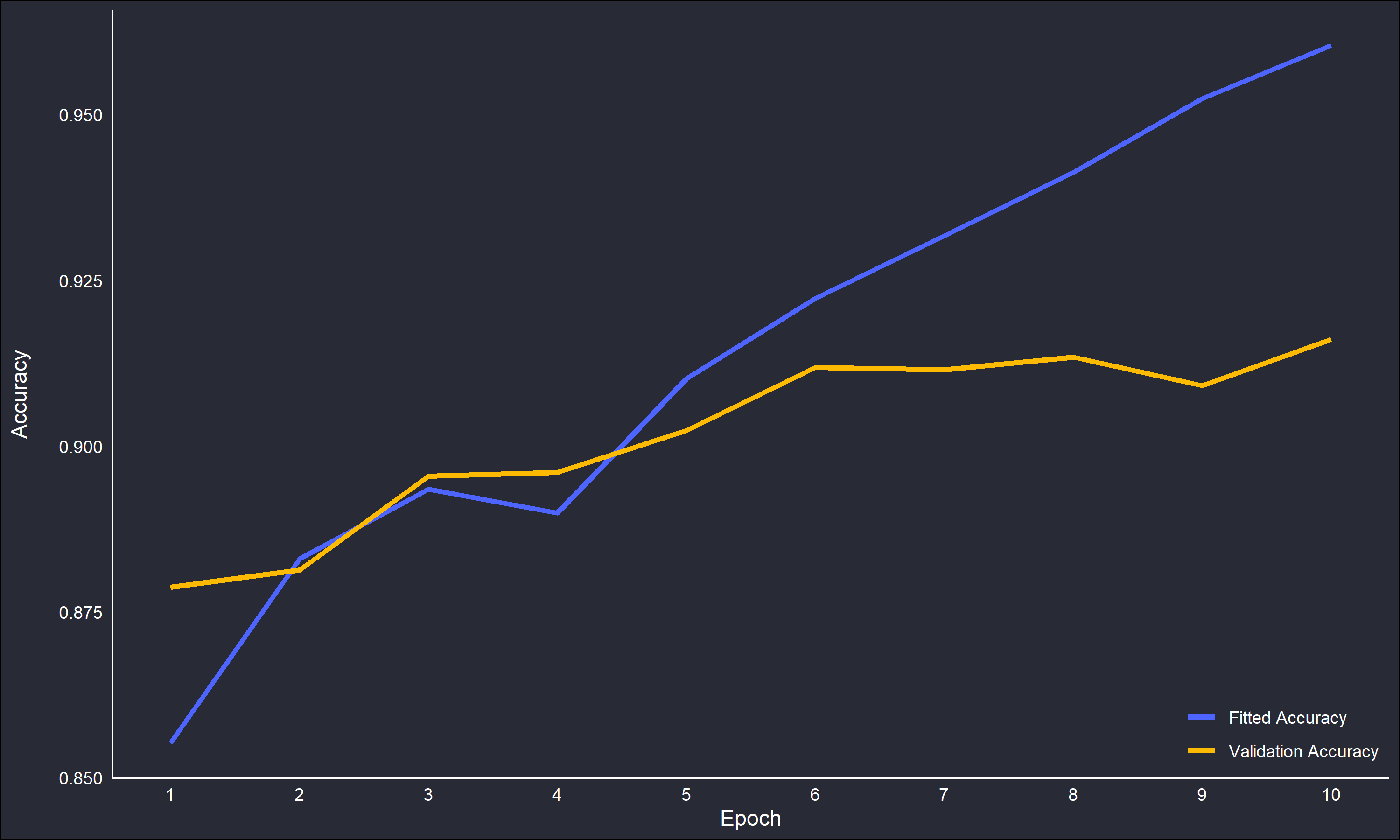
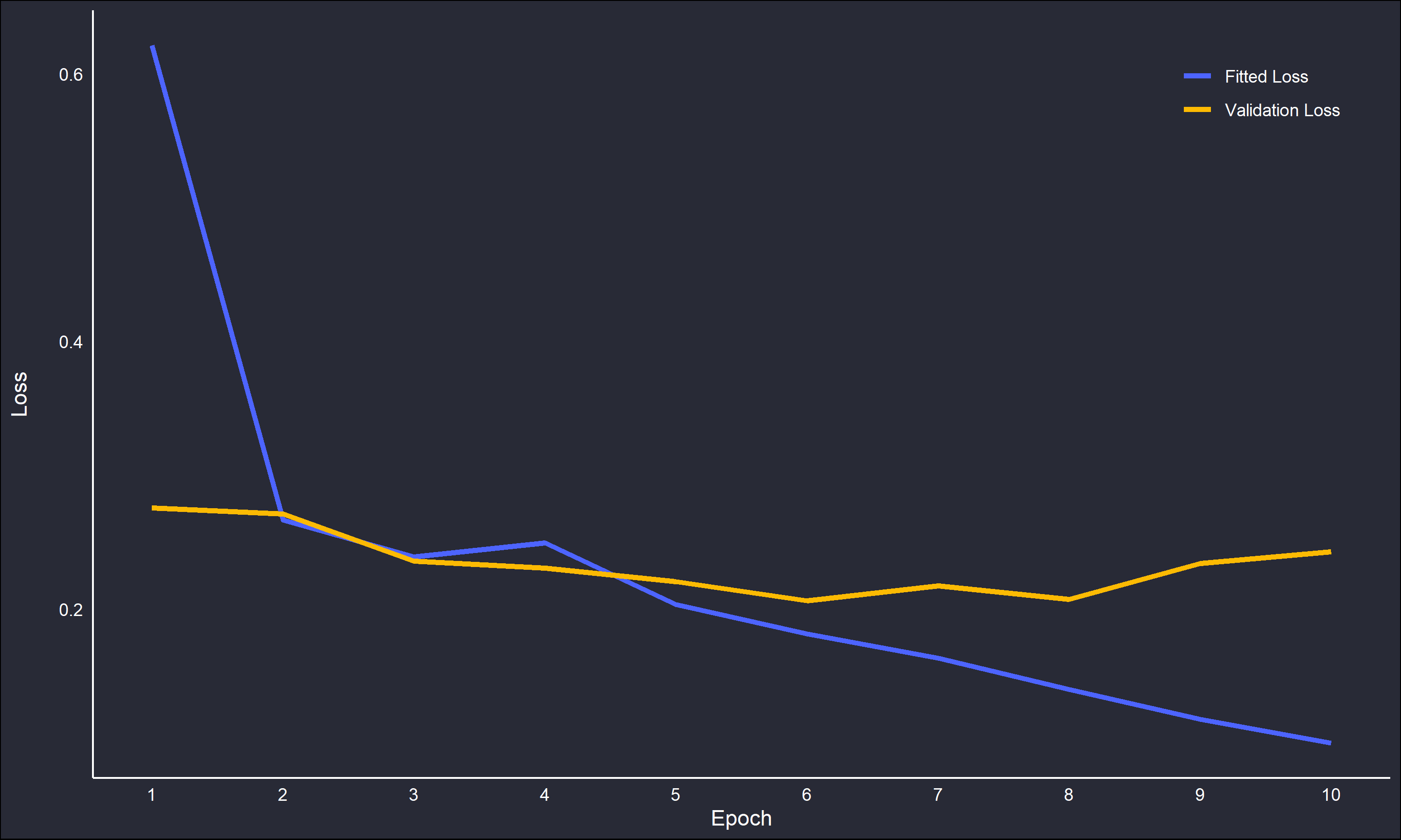
The “accuracy” variable measures how often predictions equal the correct labels. The “loss” variable is the output of the loss function, the mathematical object that is being optimized over iteratively. The accuracy for the fitted model increases more rapidly than over the validation set, however both are increasing. This is promising, there is likely some overfitting but nothing out of hand. However, the loss has a clear negative trend for the fitted model but a much flatter trend for the validation set, and actually is increasing at the later epochs.

As a final assessment of the Chess CNN model, I took 10 non-checkmate and 6 checkmate positions from the pool of positions that were not used as training or test data, and fed them into the model to see how it did.

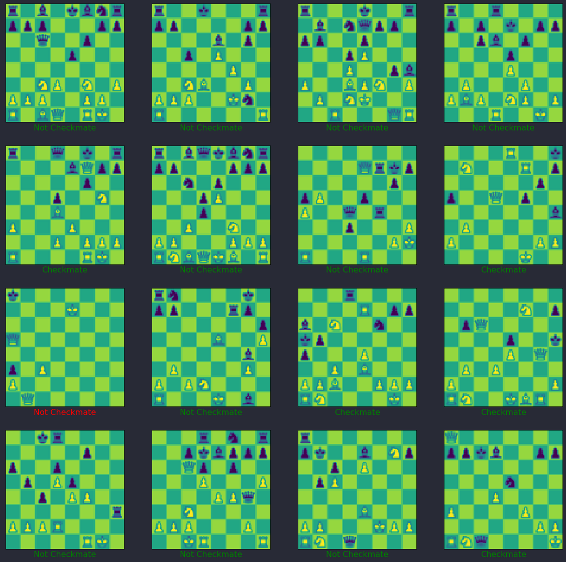
Note the actual chess positions pictures look funny because you are seeing it as the CNN “sees” them, scaled down to 100x100 pixels and in grayscale (falsely coloured by python). The results are pretty good, with 15/16 positions correctly identified (in green) and a single position (in red) misclassified. It is interesting that the single misidentified position is a checkmate. It could be interesting to look more closely at the frequency of types of misidentified positions, ie checkmate positions classified as not and vice-versa.