The Slutzky-Yule effect and the risks of smoothing data
Time series, autocorrelation, and random noise
Data measured such that successive observations are indexed by time is a time series. Time series data are not restricted to any particular scale, the only requirement is that each observation be associated with a successive point in time. This distinction enforces a natural ordering to the data; time (for these purposes) is linear and any data point in such a series will have a distinct position within the series.
Treatment of time series data is affected by this ordering that a linear conception of time imparts. In the statistical analysis of non-time series data a common assumption is one of independence, any one data point is not dependent on another. However, time series data may have past values as predictors of future values. That is, there exists correlation between data points, in other words autocorrelation.
The autocorrelation between observations of a time series \(y_t\) and lagged observations \(t-k\) is commonly denoted by \(\rho_k\). The autocorrelation is a ratio of the covariance (\(\gamma\)) between \(y_t\) and \(y_{t-k}\) and the variance of \(y_t\). A closely related measure of dependency is partial-autocorrelation, which is simply the correlation between two observations accounting for all intermediary data. In symbols,
\[\begin{aligned} \mathrm{corr}(y_t,y_{t-k}) = \rho_k = \frac{\gamma_k}{\gamma_0} = \frac{\mathrm{cov}(y_t,y_{t-k})}{\mathrm{cov}(y_t,y_t)}\\ \mathrm{corr}(y_t,y_{t-k}|y_{t-1} \dots y_{t-k+1}) = \nu_{kk} \end{aligned}\]
The computation of the partial-autocorrelation is not as simplistic as the autocorrelation, so details are omitted. Having the sample autocorrelations and partial-autocorrelations be a function of the lag \(k\) (known as ACF and PACF respectively, collectively referred to as correlograms) can reveal the underlying dependency structure within the time series. The PACF in particular is useful in “filtering” the noise from carry-over autocorrelations to better identify dependency at specific lags. It is easiest to plot the ACF and PACF and visually inspect to suppose the underlying dependency structure.
Random noise as a time series is a set of IID observations from some probability distribution. There should be no statistically significant dependency structure observed within such a series. In symbols this is modeled as,
\[ y_t = \varepsilon_t, \quad \varepsilon_t \sim F(\boldsymbol{\theta}) \]
where \(F\) is some distribution and \(\boldsymbol{\theta}\) is a vector of parameters. To illustrate the above process, 500 realizations from the standard normal distribution \(N(\mu=0,\sigma^2 = 1)\) were simulated.
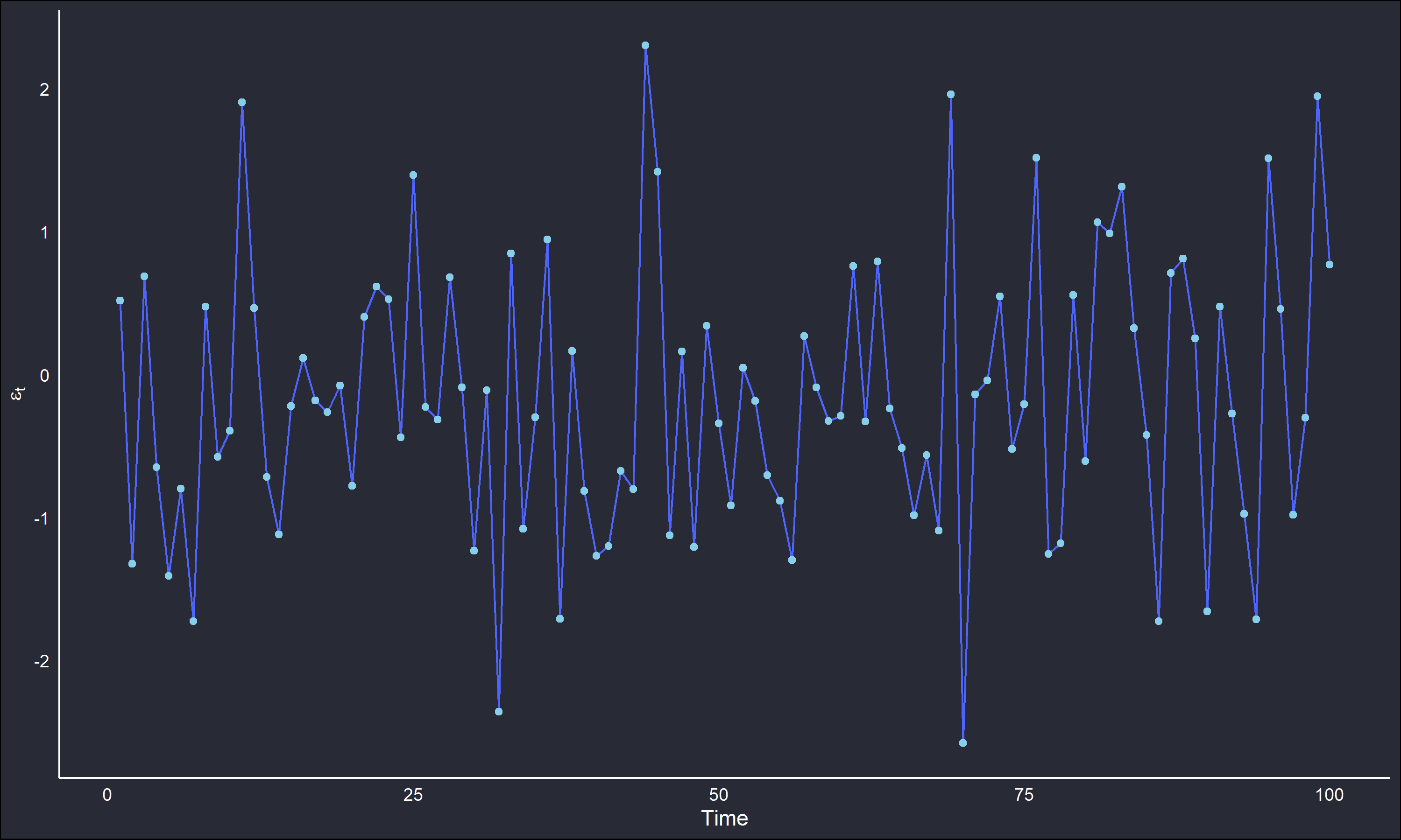
Note the stable behaviour about the distribution’s mean, there is no discernible trend or pattern that suggests dependency. Consequently, when looking at the ACF and PACF plots of the series there should be no “spikes” apparent.
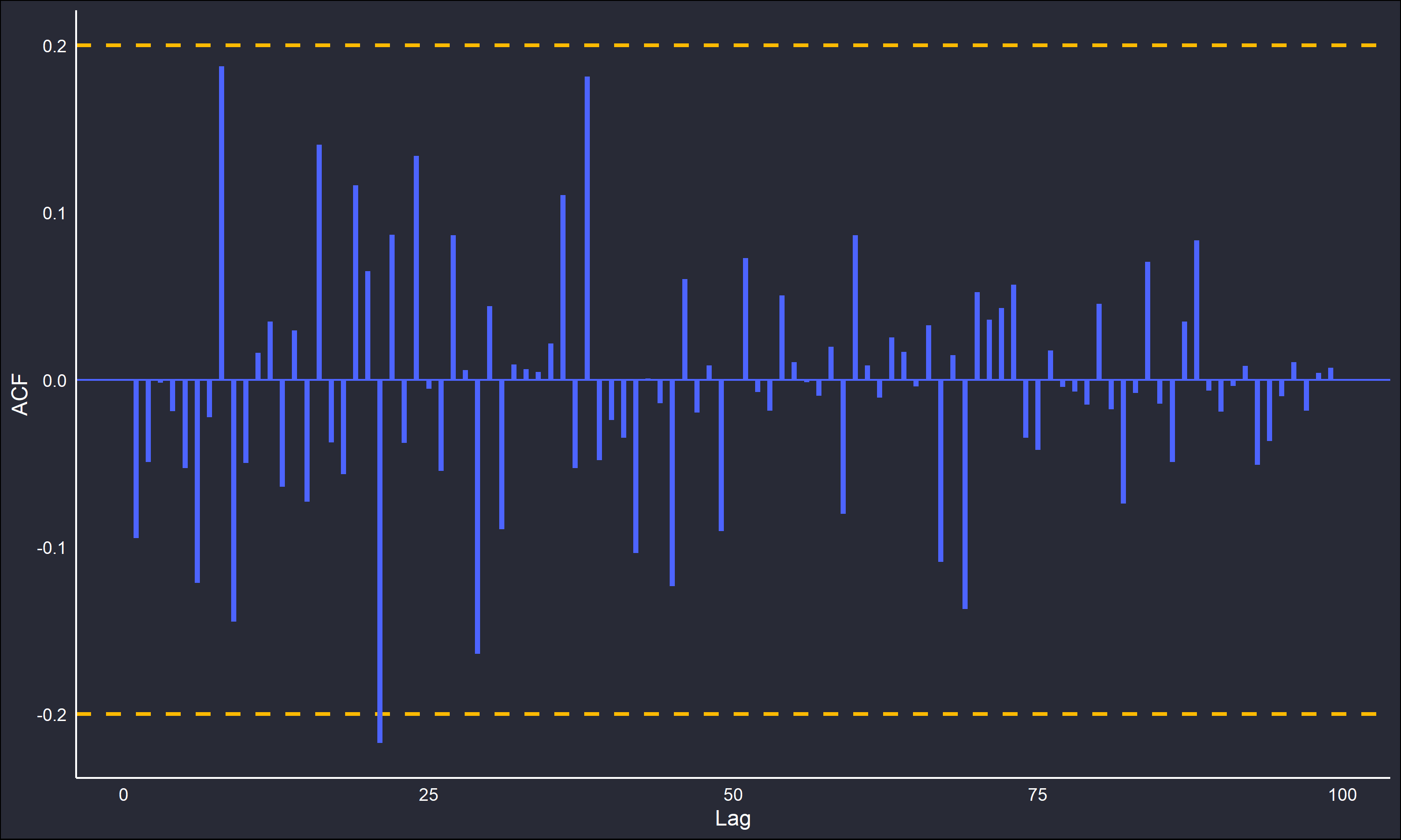
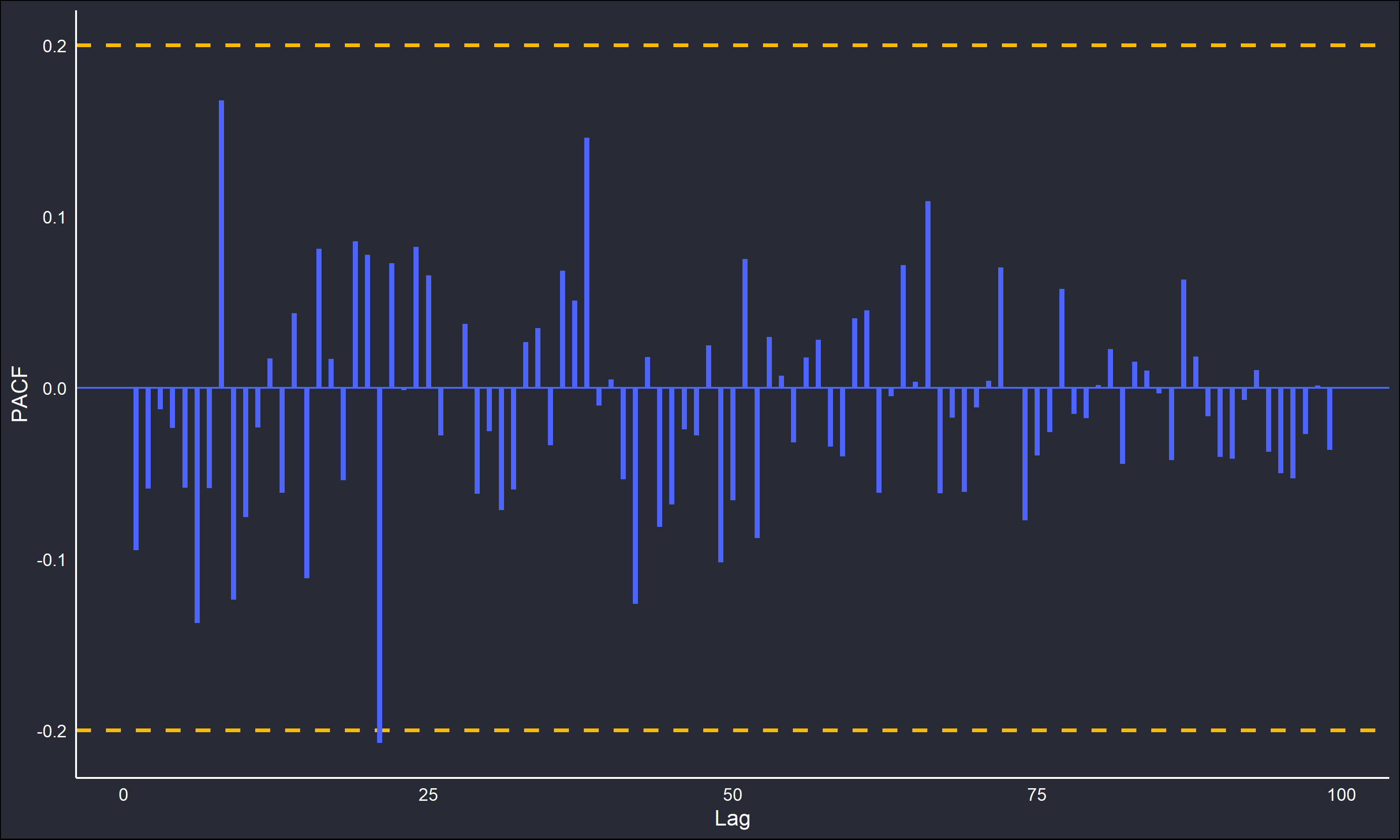
The correlograms do confirm this. Note the dotted lines, these are 95% confidence intervals to better identify any dependency. A purely random IID series will have an approximate standard deviation of \(n^{-1/2}\), with the distribution of \(\rho_k\) asymptotically normal. Details on the derivation are far beyond the scope of this post, but chapter 7 in Time Series: Theory and Methods by Brockwell and Davis is a good reference.
Slutzky-Yule Effect
The Slutzky-Yule effect was noted when observing the behaviour of a random series of observations after applying a linear operator. It was noted that linear operators (such as a moving average) would transform the random series into a series with a dependency structure. IE common smoothing techniques would induce structure that was non-existent in the underlying data.
Consider a simple moving average across the random series \(y_t = \varepsilon_t\) from earlier. Applying the filter \(\frac{1}{k}\sum_{j=0}^{k}\varepsilon_{t-j}\) to a series of length \(n\) we get a new series equivalent to the model
\[\begin{equation*} y_t = \varepsilon_{t-k} \end{equation*}\]
which has dependency at lag \(k\) and a length of \(n-k\). Dependency in the error is referred to as a Moving Average (MA) structure, whereas dependency in the variable of interest is known as an Autoregressive (AR) structure. Hence the above equation is an MA(k) moving average structure, born from a series of pure noise.
To illustrate this, a moving average of length 2 (\(k=1\)) was applied to the random noise generated beforehand. The smoothed time-series, as well as the ACF and PACF are plotted below.
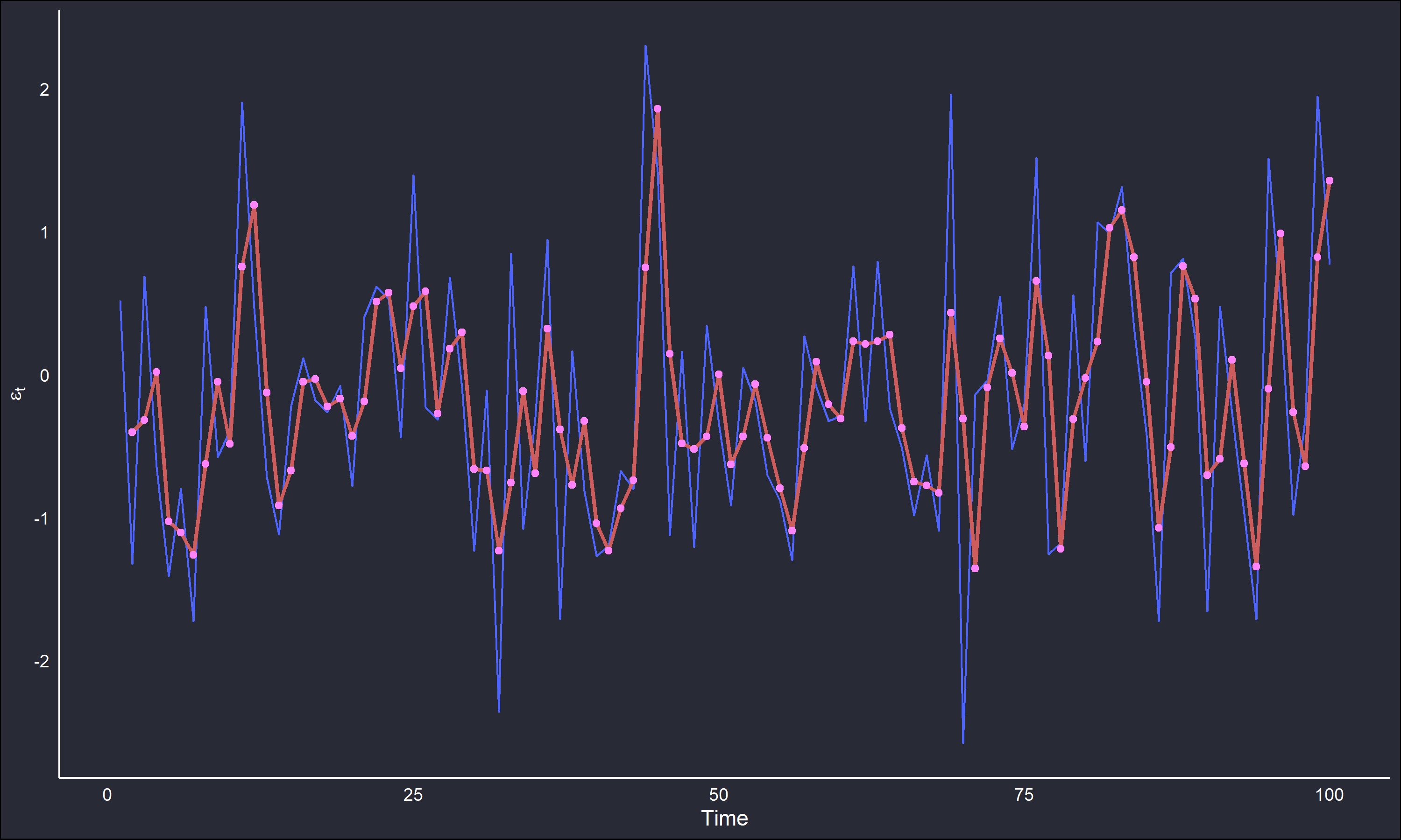
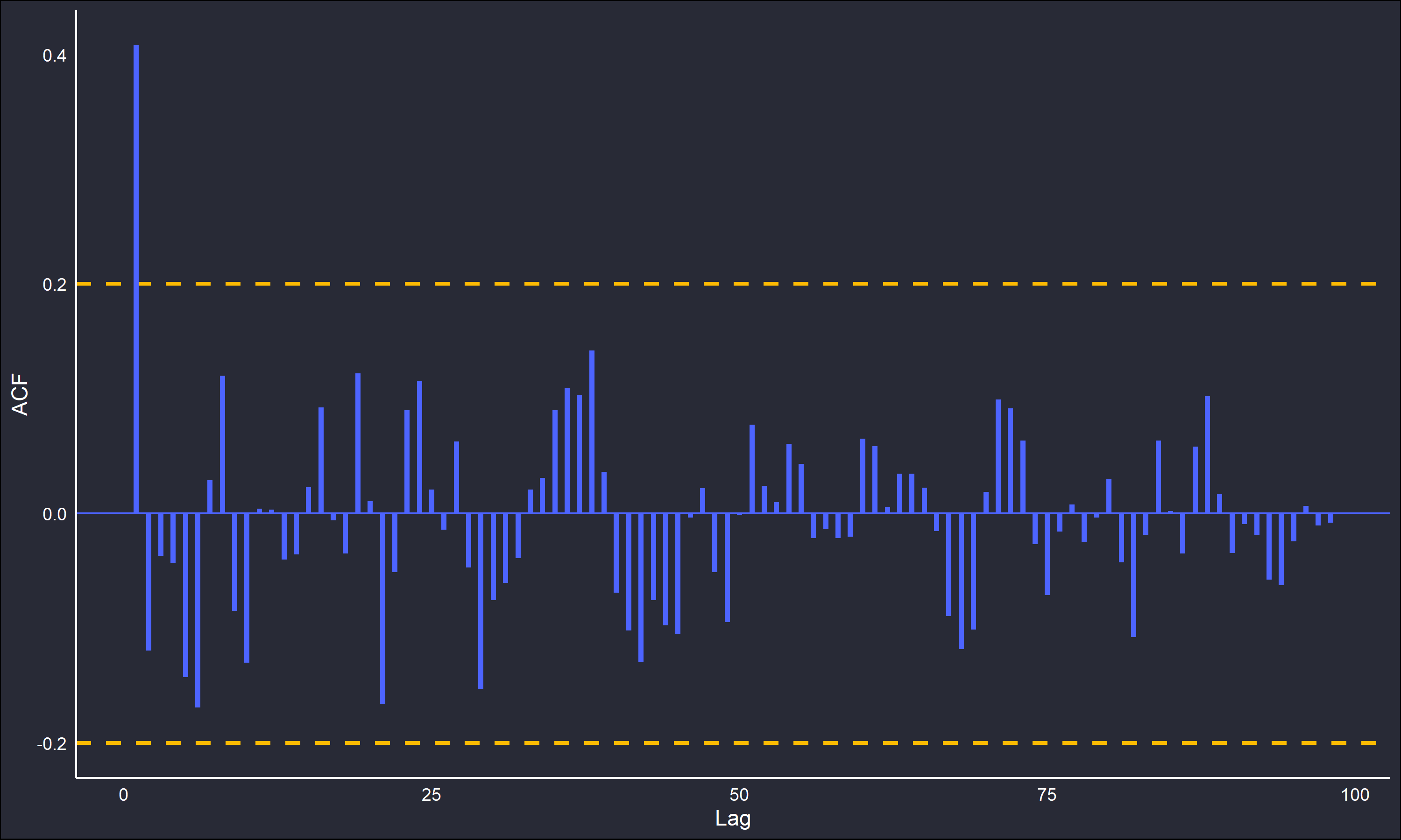
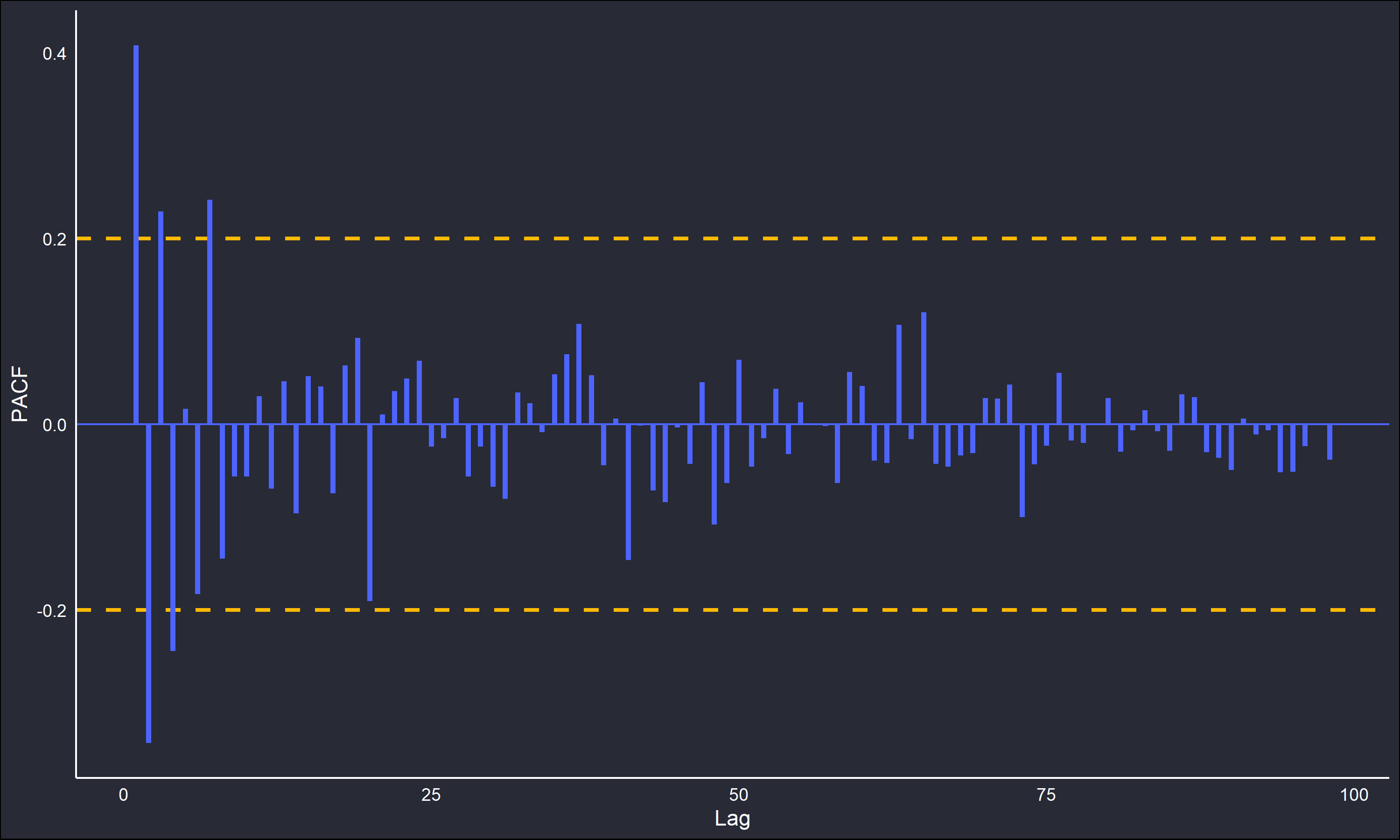
The correlograms show behaviour expected of a MA(1) series; the single spike at lag 1 in the ACF and the oscillating decay in the PACF are highly typical of this structure. Even with the most minimal possible averaging, a dependency structure was still induced.
The dangers of this effect are clear. Naively applying smoothing techniques to data that are strongly contaminated with random error can create an artificial structure that is misleading. The Slutzky-Yule effect illustrates the importance of having a good grasp of the data being analyzed, and the process that generates it, before making any transformations. Moving-averages and other linear filters are useful in cutting through noise and capturing underlying signals, but only when a strong enough signal is present. Otherwise you are chasing ghosts.