Robust estimators
In statistics, an estimator that is robust is one that is resistant to violations in an assumed parametrization of data. In practical terms this often corresponds to observations in a dataset that are not readily explainable by any known underlying model. In other words outliers that cannot be accounted for.
In such situations it may be desirable to reduce the effect of outliers in any subsequent analysis rather than discarding the data completely. Discarding data is generally inadvisable, and should only really be done if the underlying process behind undesirable datapoints is well understood.
To illustrate the potential undesirable effects outliers may have on a dataset, I will look at two very well-known estimators of location, the mean and the median.
The mean is defined as,
\[ \bar{x} = \frac{1}{n}\sum_{i}^{n} x_i \]
the median as,
\[ \text{Med} = ((n+1)/2)^{\text{th}} \text{ value of ordered set } x_i \]
for some data set \(\mathbf{x}, \ x_i \in \mathbf{x}\).
The mean is clear. In simplest terms, the median is calculated as the middlemost value of an ordered dataset. If a dataset has an odd number of observations this will be just the middle number. If a dataset has an even number of observations the median will be taken as the mean of the two middlemost values.
Returning to the concept of robustness, notice for the mean every \(x_i\) in the summation carries the same coefficient, 1. Every observation of the data \(x_i\) is weighted the same in the estimate. This can lead to even a single outlier having an out-sized effect on the mean as an estimate. Conversely, the median is calculated based on the ordered set of the data, a single outlier will have no more effect than any other single observation.
To illustrate this, consider the toy dataset \(\mathbf{x} = \{9.2, 8.8, 11.1, 33.0, 10.7\}\). Using the formulas for the mean and median,
\[\begin{equation*} \bar{x} = \frac{9.2+8.8+11.1+33.0 + 10.7}{5} = 14.56 \\ \end{equation*}\]
\[\begin{equation*} \text{Med}(\mathbf{x}) = ((5+1)/2)^{\text{th}} \text{ observation of } \{8.8,9.2,10.7,11.2,33.0\} = 10.7 \end{equation*}\]
The mean gives a value greater than 4 of 5 values in \(x_i\), whereas the median provides a more “expected” value relative to the majority of observations. In a real dataset, a clear outlier such as \(x_4\) could greatly skew the mean from the majority of the data. In some situations this may be desirable, as the outliers could be well understood processes that should be priced into any estimates of location, but in many situations outliers serve only to skew estimates undesirably.
To further explore this concept, I’ll do some simple simulations.
Simulation 1
Consider \(\mathbf{x} = x_i \sim t(v = 2), \ i = \{1, \dots,n=50\}\), where \(t\) is Student’s t distribution parametrized with \(v=2\) degrees of freedom. Like the normal distribution, the t distribution is symmetric and “bell” shaped. However, it has heavier tails than the normal distribution, especially with \(v=2\). It also is centered about 0, so any estimate of location should be \(\approx\) 0. The sample \(\mathbf{x}\) has outliers shown in the below figures.
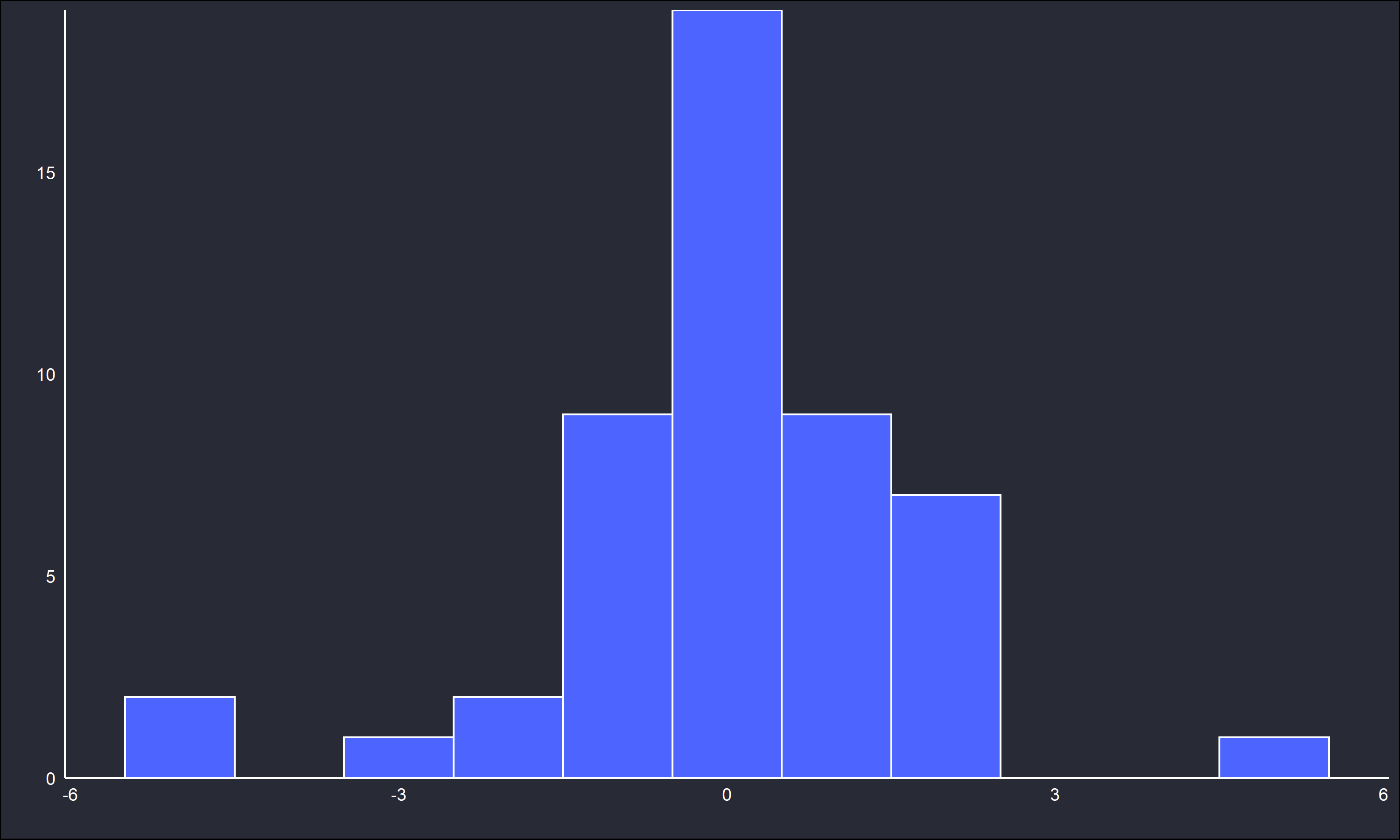
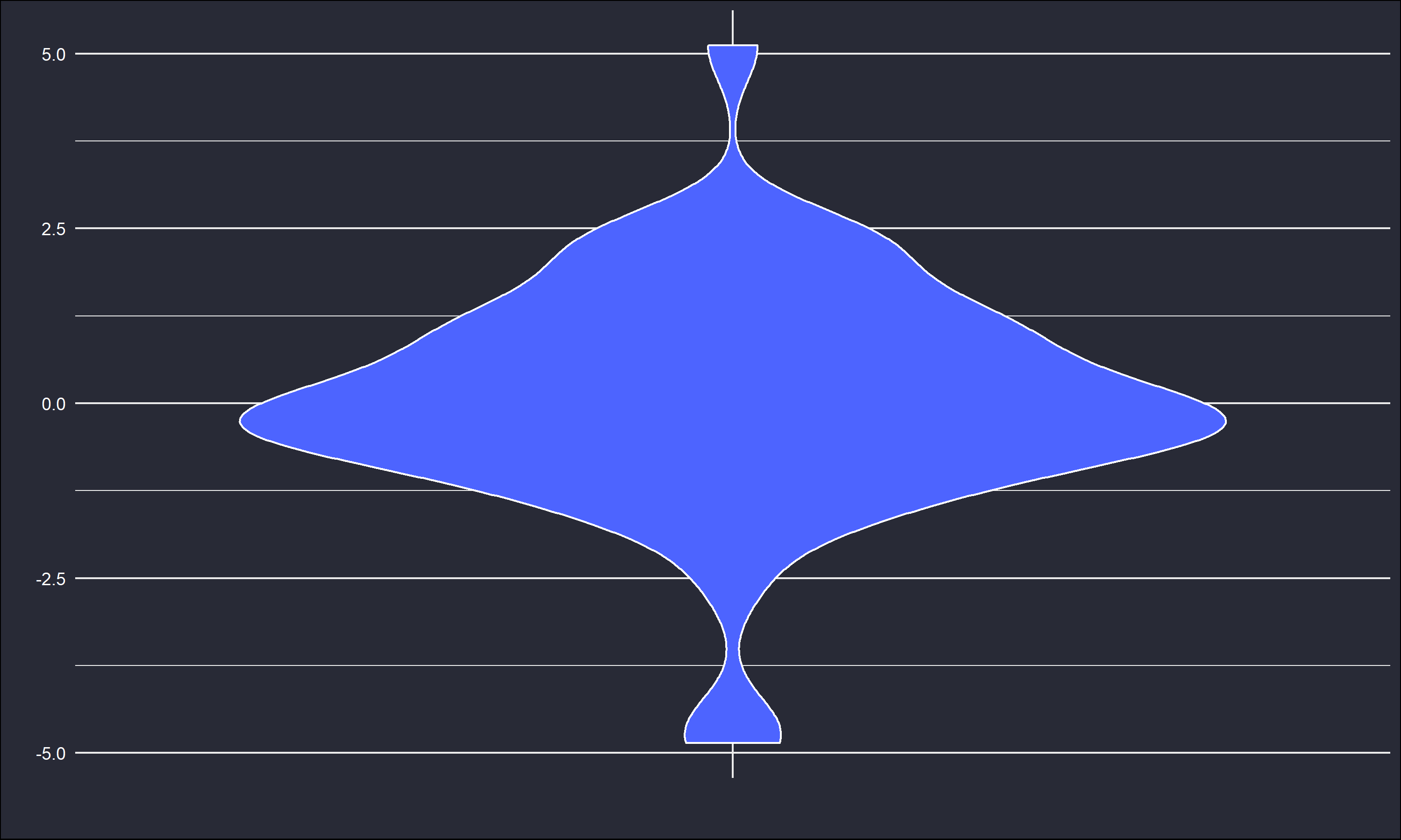
There are outliers around -4 and 6, where the majority of the observations fall about [-2,3]. Checking the sample mean and median give \(\bar{x} = 0.0905, \ \text{Med} = -0.0331\). The sample median is closer to the true center of 0 than the sample mean. Simulation can further illustrate the insensitivity of the median (and sensitivity of the mean) to outliers.
1000 replications of \(x_i \sim t(v=2), \ n=50\), are sampled, and the means and medians are calculated for for each replication’s sample. The below figures show the overlaid histograms of both estimates and a QQ plot.
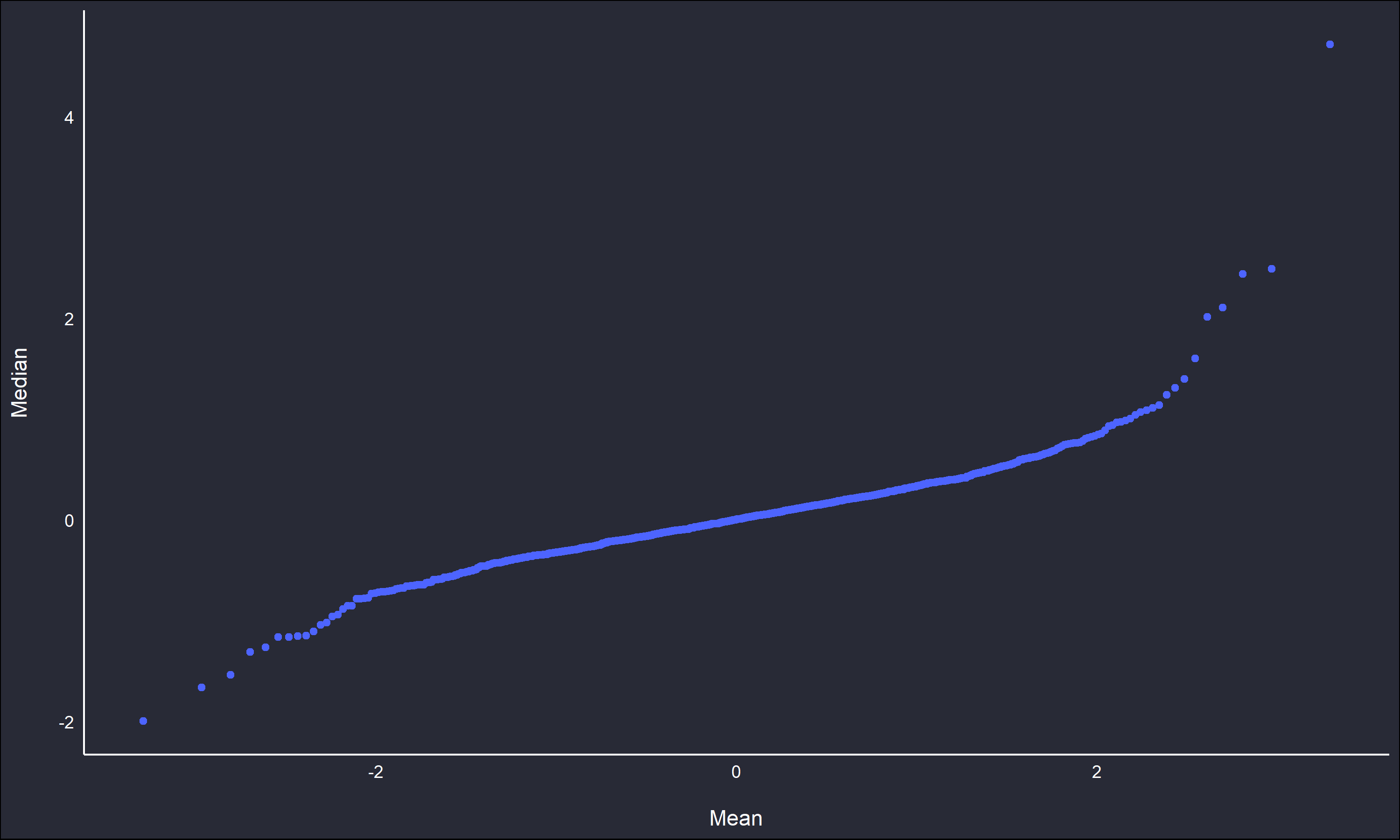
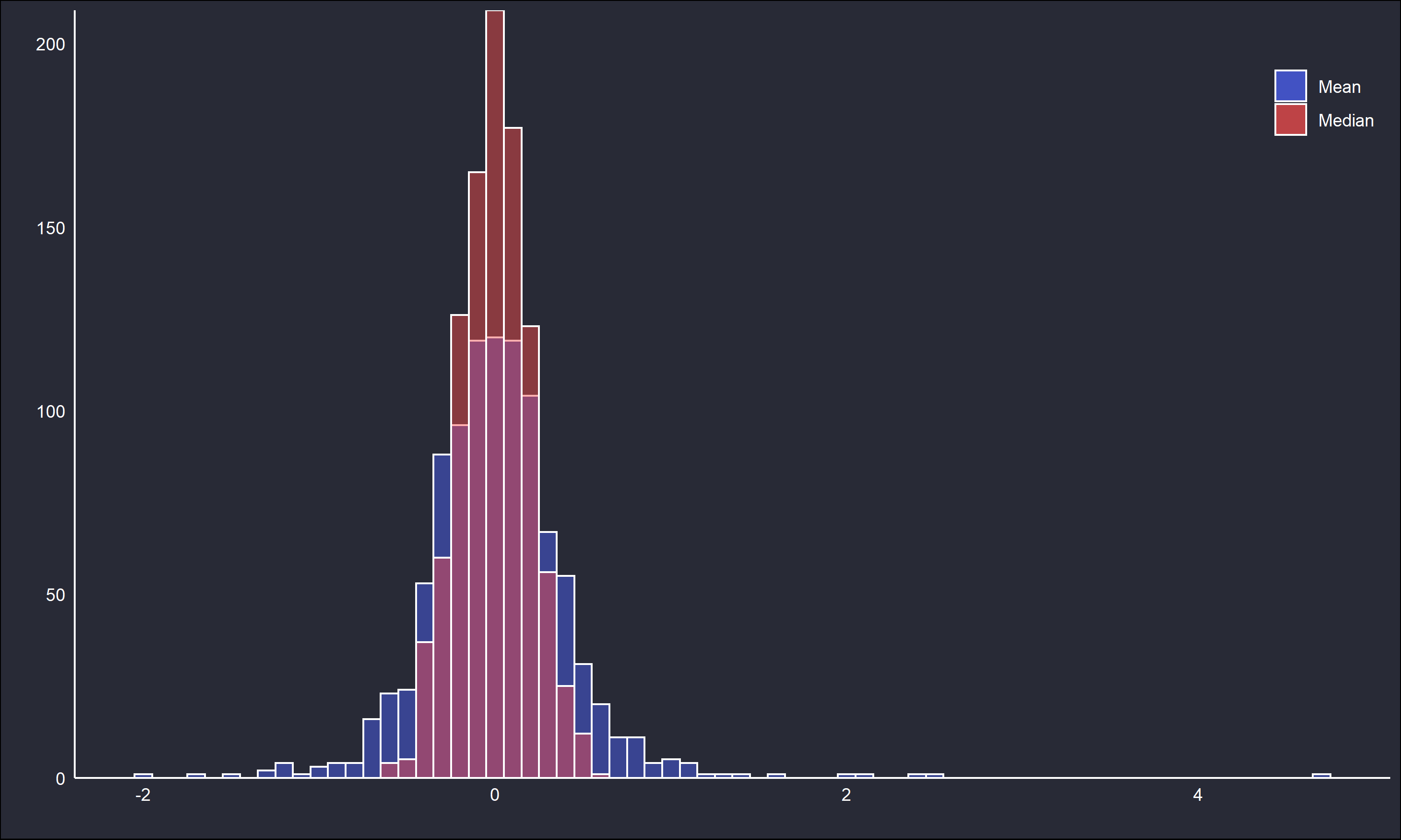
The histogram and QQ plot clearly show the median estimates are denser about the theoretical central location, and less variable than the mean estimates.
The relative value of the mean and median estimators can be conveniently assessed in a single value, the Mean Squared Error (MSE). MSE is defined as,
\[\begin{equation*} \text{MSE}_{\hat{\theta}} = \frac{1}{n} \sum (\hat{\theta} - \theta)^2 \end{equation*}\]
where \(\theta\) is the known value, and \(\hat{\theta}\) is the estimated value. The MSE takes the average squared difference between these two quantities. MSE values closer to 0 imply a better “quality” of estimator. Much more can be said on the general topic of error functions, particularly the relationship between MSE, bias, and variance, but for this post let’s leave it here.
Calculating the MSE for the replicated means and medians gives \(\text{MSE}_{\bar{x}} = 0.181, \text{ MSE}_{\text{Med}(x_i)} = 0.039\) respectively. In this case \(\theta\) is 0 as this is the center of the considered t distribution. Clearly the median is a better estimator according to the chosen error function.
Simulation 2
In simulation 1 all the replicates were of a fixed sample size, \(n = 50\). It could be interesting to see how the estimators perform across gradually larger sample sizes. 1000 replications of \(x_i \sim t(v=2)\) for fixed increments of \(n = \{50, 100, 150, \dots, 1000\}, \ i = \{1,\dots,n\}\), will be considered. The MSE of estimators will be plotted as functions of \(n\) to discern how sample size may affect the estimate’s “quality”.
In addition to the mean and median, I have coded a crude weighted estimator of the mean (for a distribution centered about 0) to consider in the simulation as well. The weighted mean is defined as such,
\[\begin{equation*} \hat{\text{W}} = \frac{1}{n}\sum_{i}^{n} w_ix_i, \begin{cases} w_i = 1, & \text{if $x_i \in [-\frac{1}{2\bar{x}s_x}, +\frac{1}{2\bar{x}s_x}]$} \\ w_i = \frac{1}{2} & \text{otherwise}. \end{cases} \end{equation*}\]
where \(s_x\) is the sample standard deviation of a sample \(x_i\).
Performing the simulation…
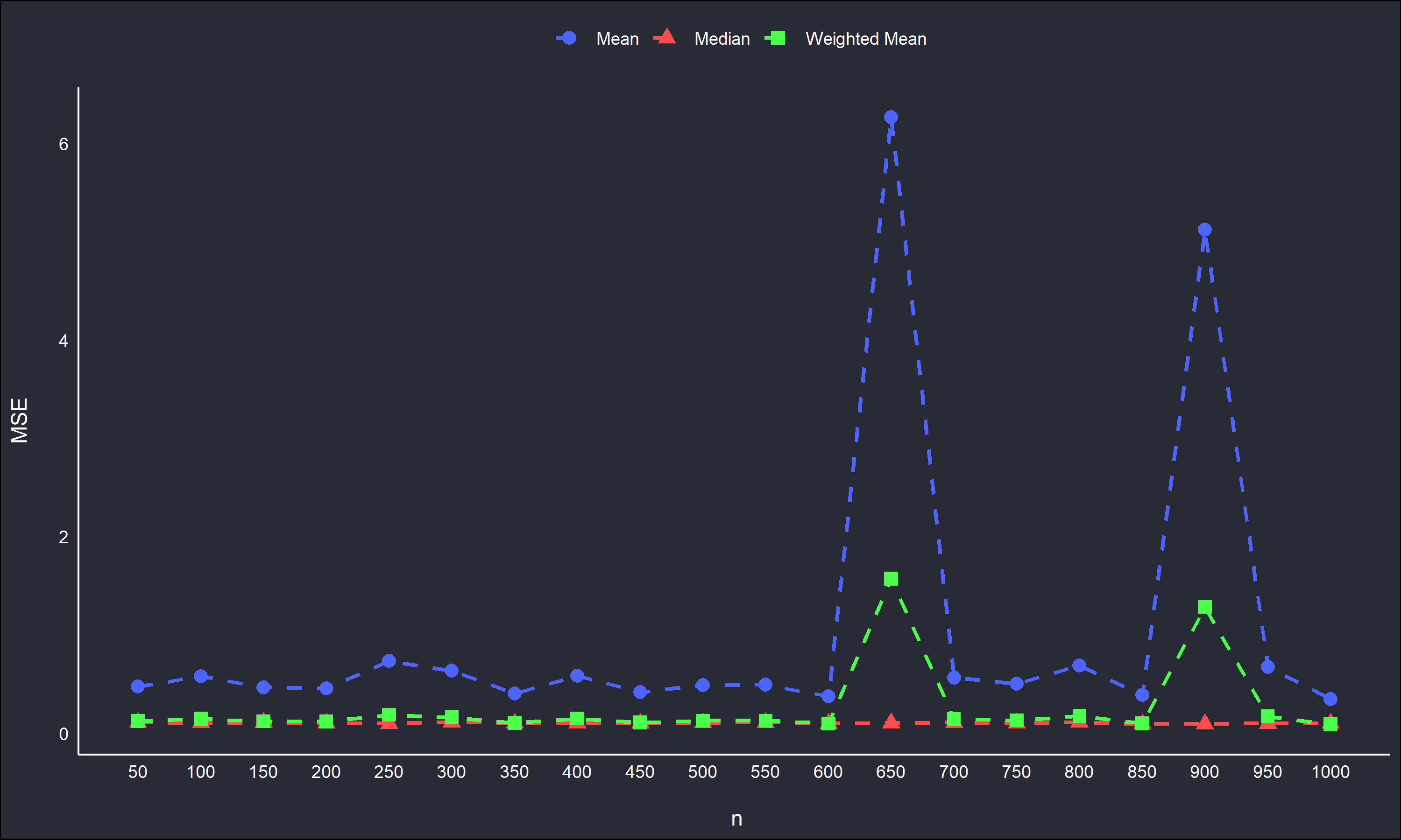
The median is the most stable estimate, hovering around a MSE of 0 as \(n \to 1000\). The crude weighted mean is also surprisingly stable, except at \(n = 650\) and \(900\), which also correspond to large spikes in the typical sample mean. This is likely due to these replication blocks randomly containing more outliers in one tail of the samples than the other. The typical sample mean will be severely affected, and the weighted mean cannot account for more outliers in one tail over another. It is interesting this occurred in replication blocks for relatively large \(n\).
Zooming in on the MSE estimates give a useful plot as well.
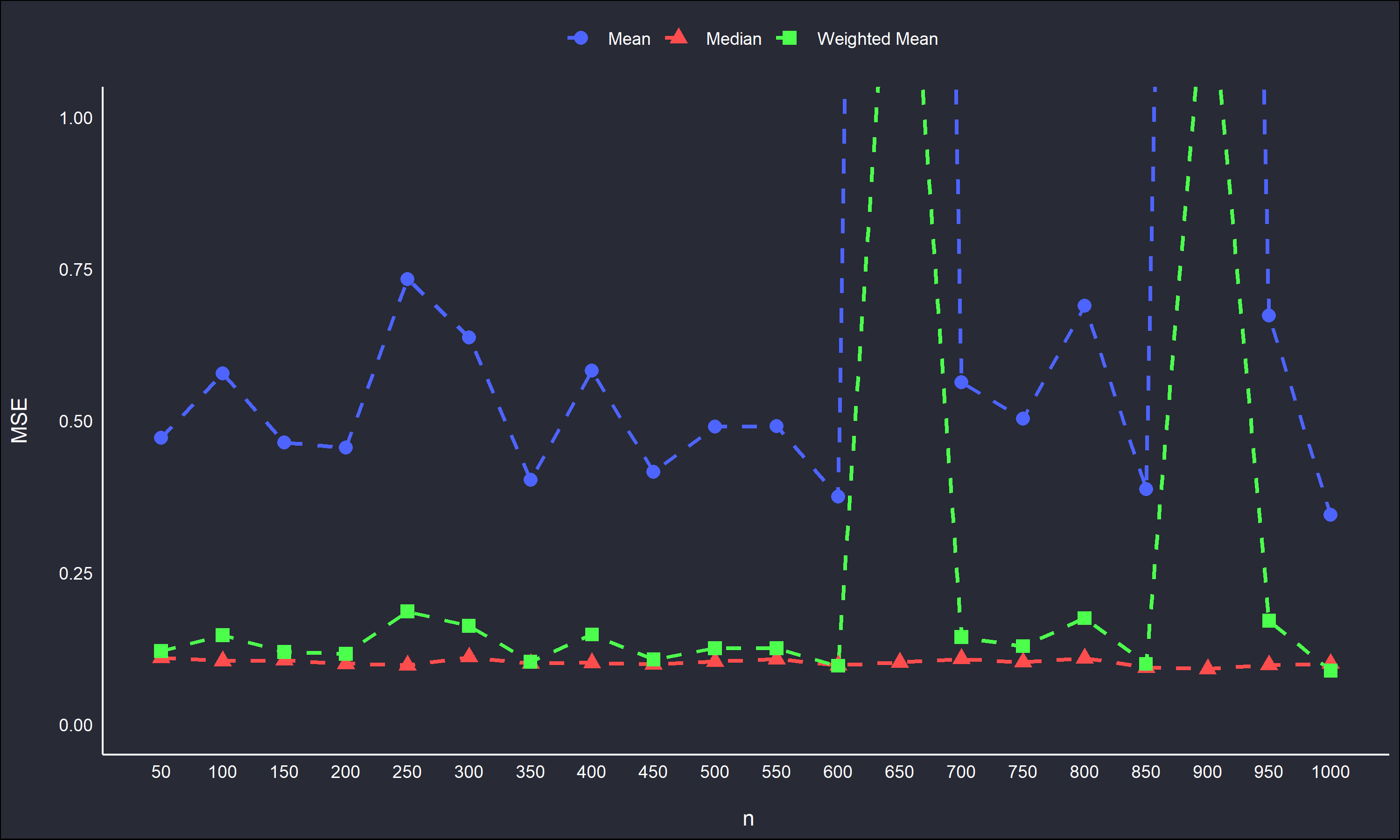
By cropping the out-sized MSE values, it is more clear that the weighted mean usually underperforms the median with respect to MSE, and the typical sample mean MSE is quite variable across \(n\). The median is the most stable estimate with respect to MSE.